Revisiting Ice Ages Cycles

Abstract

The astronomical theory of ice ages is widely accepted. Yet, it is not abundantly clear just exactly what the astronomical theory of ice ages is, other than the vague statement that variations in the Earth's orbit produce changes in solar irradiance at northern latitudes which is somehow related to the formation and termination of ice ages. Periodic variations in the Earth’s orbit produce variations in the insolation at high latitudes and ice ages begin on down lobes of insolation and terminate on up lobes of insolation. However, not all down lobes create ice ages and not all up lobes produce terminations. The ice ages changed character at the so-called mid-Pleistocene transition, about a million years ago. There is no current physical explanation for these difficulties with the astronomical theory. A reasonable explanation has been developed, that solidifies the astronomical theory by explaining the rise and fall of ice ages in both eras. The solar power absorbed at high northern latitudes depends on the insolation and absorptivity of the surface. The absorptivity is particularly affected by the obliquity in the pre-MPT era, and by dust deposits late in the post-MPT era. When these are included, it can be explained why some down lobes produce ice ages, and some up lobes produce terminations in both eras. In the pre-MPT era, ice ages originate when the insolation enters a down lobe and the obliquity is minimal (higher reflectivity) and ice ages terminate at a coincidence of high insolation and high obliquity (lower reflectivity). These links between SIHL and obliquity tend to be repetitive with approximately 41,000-year spacing. In the post-MPT era, ice ages also originate at a down lobe of SIHL. However, once an ice age is started, each successive up lobe in SIHL might cause a slight decrease in ice volume but doesn’t bring about a termination. After several precession cycles, high dust levels increase absorptivity, and the next-up lobe produces a termination.

Introduction

It is widely accepted that variations in insolation to high latitudes are the driving force for the observed periodic occurrence and termination of ice ages. This paper provides rationalizations for why some increases in insolation to high northern latitudes produce terminations and some do not, and why some decreases in insolation to high northern latitudes induce ice ages, and some do not. It also provides a rationale for why the spacing of ice ages changes across the Mid-Pleistocene Transition (MPT).

Background

Rapp (2018) provided an extensive summary of experimental data and modeling of ice ages [11Rapp D. Ice Ages and Interglacials. Heidelberg: Springer-Praxis Books; 2018.]. Experimental data from ice cores [22Masson-Delmotte V, Buiron D, Ekaykin A, et al. A comparison of the present and last interglacial periods in six Antarctic ice cores. Clim Past. 2011;7:397-423.] and ocean sediments [33Rapp D. Ice Ages and Interglacials. Heidelberg: Springer-Praxis Books; 2018. Section 1.] reveal the buildup and decline of giant ice sheets in high northern latitudes over the last few million years. Physical evidence such as ice sheet moraines, coral terraces, and surface variations support these findings [44Rapp D. Ice Ages and Interglacials. Heidelberg: Springer-Praxis Books; 2018. Section 6.]. In addition, spectral analysis of the ice data shows fundamental frequencies that mirror the frequencies of solar variations [55Rapp D. Ice Ages and Interglacials. Heidelberg: Springer-Praxis Books; 2018. Section 9.2.]. There is little doubt that quasi-periodic variations in the Earth's orbit cause variations in SIHL, which are the pacemakers for the initiation and decline of ice ages. However, the specific connection between variations in SIHL to variations in global ice volume remains unclear. In this section, I review several references that are relevant to this issue.

The character of ice ages changed across the Mid-Pleistocene Transition (MPT) about one million years ago. Before the MPT, ice ages did not accumulate as much ice and were spaced at roughly 41,000-year intervals. After the MPT, ice ages accumulated more ice and were spaced at wider intervals ranging from 88,000 years to 110,000 years. A large body of experimental data and analysis has clearly shown that variations in insolation at high northern latitudes play an important role in determining the timing of ice ages in both eras. Spectral analysis of ice volume variability data displays the cadence of insolation [66Muller RA, MacDonald GJ. Ice Ages and Astronomical Causes. London: Springer Publishing Co.; 2002.].

Periodic variations in the Earth’s orbit produce variations in the insolation at high latitudes [77Berger WH, Loutre MF. Insolation values for the climate of the last 10 m.y. Quat Sci Rev. 1991;10:297-317.], and ice ages begin on down lobes of insolation and terminate on up lobes of insolation. However, not all down lobes create ice ages and not all up lobes produce terminations. The ice ages changed character at the so-called mid-Pleistocene transition, about a million years ago. Until now, there has not been a fully satisfactory explanation for these exceptions. I have developed a reasonable explanation that solidifies the astronomical theory by explaining the rise and fall of ice ages in both eras.

In this article, we define the insolation falling on the unit area (above the atmosphere) at a high northern latitude (typically 65 °N) as the “Solar Input to High Latitudes” (SIHL). Variations in the Earth’s orbit about the Sun produce periodic oscillations in SIHL. The SIHL oscillates in time due to precession with a period of about 21,000 to 22,000 years. The amplitude of these oscillations is determined by the variable obliquity (41,000-year period) and eccentricity (~100,000-year period) of the earth’s orbit. A plot of SIHL vs. time shows primary oscillations with the period due to precession, with the amplitude of the oscillations determined by obliquity and eccentricity at any time point.

The purpose of this paper is to examine the relationship between SIHL and the ice age cycles (separately for pre-MPT and post-MPT) and to thereby provide a rationalization for how up lobes and down lobes of SIHL affect the ice age cycles in each era.

Several investigators have attempted to explain at least partially why the pattern of ice volume vs. time does not reflect the timing of the rapidly varying SIHL. Rapp (2018) discusses several theories. One appealing approach is to create a differential equation where the key dependent variable is the global ice volume and the main dependent variable is the SIHL. The SIHL has been estimated and tabulated by year over millions of years. The hope would be that the known variation of SIHL with time [77Berger WH, Loutre MF. Insolation values for the climate of the last 10 m.y. Quat Sci Rev. 1991;10:297-317.] would lead to predictable variations in global ice volume (V) with time. The major challenge in explaining the timing of ice volume driven by variability of SIHL is the fact that SIHL oscillates up and down with a period of 21,000 to 22,000 years due to precession, while the pattern of ice volume vs. time shows much longer periods and does not display the oscillations of precession. What is observed (both pre-MPT and post-MPT) is that every initiation of an ice age occurs in sync with a down lobe of SIHL, and every termination of an ice age occurs in sync with an up lobe of SIHL. The problem is that not every down lobe initiates an ice age and not every up lobe terminates an ice age. And it is not clear a priori why that is so [11Rapp D. Ice Ages and Interglacials. Heidelberg: Springer-Praxis Books; 2018.].

A few key papers that utilized differential equations based on physics to predict ice volume from SIHL are reviewed next. A major challenge in these models is to obtain a pattern of ice volume vs. time that shows a slower variation than the variation of precession that governs SIHL. In addition, a recent paper that suggests an alternative to astronomical theory is briefly reviewed.

Simplest model (1980)

Imbrie and Imbrie (1980) proposed a simple formula for modeling the effect of variations of SIHL on ice volume in the post-MPT era [88Imbrie J, Imbrie JZ. Modeling the climatic response to orbital variations. Science. 1980;207:943-953.]. They formulated dV/dt as the rate of change of global ice volume and defined the deviation from the long-term average SIHL as "S". When S > 0, the SIHL tends to reduce ice volume, and when S < 0, the SIHL tends to increase ice volume. Thus, they put "–S" on the right side of the equation for dV/dt, assuming the relationship is linear. They also made several embellishments to the model. They proposed the equation:

dV/dt = – {(1 ± B)/τ} {S + V}

Where S is a measure of SIHL and V is meant to be a measure of the ice volume, to be determined by integration over time. They assumed that ice ages in the post-MPT era built ever more slowly over many tens of thousands of years. Therefore, they added the term "V" to "S" on the right side of the equation to slow down the rate of buildup of "V" as "V" increases. In addition, they added the ± sign in front of a constant B and required that we use the + sign when dV/dt is negative, and the – sign when dV/dt is positive. That allows the rate of change of V with time to be slower when the ice is building up, and faster when ice is diminishing.

The term τ was included supposedly as a time-delay term, under the belief that as the driving force S changes, it takes thousands of years for the ice volume to approach a new equilibrium due to changes in S. Note that τ is measured in thousands of years, and the integration of the differential equation takes place typically over several hundred thousand years. But is  actually a time-delay term in the equation? Not really. The term τ mainly affects the magnitude of dV/dt relative to (V + S), but the timing of the ups and downs of V(t) vs. time is dictated primarily by the time-dependence of S which is the forcing equation. Since V(t) is given in arbitrary numbers, the value chosen for τ seems to be somewhat irrelevant to the model. Integration of the equation proves that τ does not produce a time delay [11Rapp D. Ice Ages and Interglacials. Heidelberg: Springer-Praxis Books; 2018.].

Mathematically, V is a quantity that obeys the above differential equation. The greater V is, the more it acts to make dV/dt less positive (or equivalently, more negative). One then interprets V as measured from its long-term average if one believes a priori that the rate of accumulation of snow/ice is inhibited by increased snow/ice, one might interpret V as being related to ice volume, although exactly what that relationship is, is not clear at the outset.

One can then tabulate S year by year for hundreds of thousands of years and integrate the above equation to determine how V varies with time. We have done this for numerous cases.

There are at least three problems with this model:

1)  In the pre-MPT era the experimental pattern of V vs. t found in the LR–04 stack of ocean sediment data is that of a series of trapezoid-like patterns, and the rate of increase of ice volume when ice growth is rapid is about the same as the rate of diminution of ice volume when decay is rapid, across any ice age in that era. So, one would think that B should be close to zero in the pre-MPT period (Figure 1).

11Rapp D. Ice Ages and Interglacials. Heidelberg: Springer-Praxis Books; 2018.]." /> Figure 1: Typical pattern of ice ages in the pre-MPT era [11Rapp D. Ice Ages and Interglacials. Heidelberg: Springer-Praxis Books; 2018.].

2)  In the post-MPT era, particularly over the four most recent ice ages, the actual pattern of V vs. t is not a slow buildup, followed by a rapid decrease (as is often assumed). The actual pattern of V(t) is a rapid buildup to perhaps half of the ultimate maximum V in 5,000 to 10,000 years, followed by a long, slow buildup to the maximum V, followed by a rapid decrease (Figure 2).

11Rapp D. Ice Ages and Interglacials. Heidelberg: Springer-Praxis Books; 2018.]." /> Figure 2: Typical pattern of ice ages in the post-MPT era [11Rapp D. Ice Ages and Interglacials. Heidelberg: Springer-Praxis Books; 2018.].

3)  The discontinuous change in the differential equation where dV/dt changes sign is not physical. It would be more reasonable to make B a continuous function of V. A hyperbolic tangent might work well.

I carried out multiple integrations of the Imbries’ equation in the post-MPT period and it produces a pattern of V(t) that varies with a ~ 22,000-year period due to precession. The calculated V(t) does not resemble the actual ice ages. In plain words, the Imbries model doesn’t work. The resulting pattern of ice volume vs. time is dominated by the rapid variations of SIHL due to precession, which is not observed in the ice volume data. Figure 3 shows the result of integrating the Imbries' equation in the pre-MPT era.

Figure 3: Calculated relative ice volume using the Imbries’ equation.

There are fundamental reasons why Imbries’ equation doesn't work well in the post-MPT era. One is that there is no reason to think that the response to S and V should be linear. It is sometimes believed that ice accumulates slowly and terminates rapidly, following a "sawtooth" pattern. The Imbries equation is based on that notion. However, inspection of the actual ice volume patterns in both the pre-MPT and post-MPT eras shows that the actual patterns do not follow that simple notion. In both eras, ice accumulates very rapidly in the first several thousand years of an incipient ice age. After that, the ice volume reaches a plateau in the pre-MPT era and slowly increases in the post-MPT era. The Imbries’ equation can't possibly account for that (Figure 2). Furthermore, there is no evidence that the value of V inhibits dV/dt in the early stages of glaciation. The rate of ice accumulation is high for several thousand years and seemingly independent of V. From a longer point of view in the pre-MPT, the variables S and obliquity determine dV/dt, and V does not necessarily enter, or if it does, it is complex .

More complex model (1998)

Paillard (1998) presented a model in which depending on the values of insolation and ice volume, the climate system would respond in three different regimes: i (interglacial), g (mild glacial), and G (full glacial), and the differential equations that govern transitions between them are constrained by rules [99Paillard D. The timing of Pleistocene glaciations from a simple multiple-state climate model. Nature. 1998;391:378-381.]. This approach is an improvement over Imbries’ model and further development of this approach might provide good insights. Rapp (2018) suggested an increase to four regimes, adding a termination regime and he analyzed how that might work. However, this approach requires further analysis with realistic data for SIHL.

As one adds parameters and defines more regimes, the model begins to appear more like curve-fitting and less like a mathematical representation of physics.

Consideration of north and south (2005, 2006)

In a landmark achievement, Lisiecki and Raymo (2005) published details from the LR-04 stack of ocean sediment data that provides estimates of global ice volume over the past several million years. That stack represents arguably the best representation of the ebb and flow of global glaciation over an extended time. The raw stack data provides estimates of δ¹⁸O vs. depth in the sediments, and is equivalent to global ice volume [1010Lisiecki LE, Raymo ME. A Pliocene-Pleistocene stack of 57 globally distributed benthic δ18O records. Paleoceanography. 2005;20-PA1019.].

Perhaps the most challenging aspect of this impressive work was converting depth to a timescale for the sedimentary data. The procedure used by L&R involved a combination of several contributing approaches. One part of this analysis involved the use of the Imbries’ model. When the Imbries’ model was applied to their data in the pre-MPT era, the result was as shown in Figure 3. I performed the integration which duplicated the result provided by L&R. The Imbries’ equation produces negative values for V(t) which seems non-physical. Note that L&R converted their V(t) to a vertical scale of δ¹⁸O (¹⁸O isotope percentage) ranging from 3.0 to 4.4, but it is not clear how they did that, or even whether that makes sense physically when V(t) is always negative. This result in Figure 3 looks nothing like the actual data for ice volume.

Raymo, et al. (2006) pointed out that the ocean sediment data measured global ice volume, rather than northern ice volume [1111Raymo ME, Lisiecki LE, Nisancioglu KH. Plio-Pleistocene ice volume, Antarctic climate, and the global delta18O record. Science. 2006 Jul 28;313(5786):492-5. doi: 10.1126/science.1123296. Epub 2006 Jun 22. PMID: 16794038.]. Before the MPT, global ice volume during the ice ages didn’t reach the high levels of the post-MPT era. They made a crucial assumption that seems credible. Here, I paraphrase their argument in my terms:

It was suggested that the ice volume in the North in the pre-MPT era was not sufficient to control the global climate. Unlike the post-MPT, the growth and decay of Antarctic ice responded to the changes in solar intensity in Antarctica. Since precession causes solar irradiance in the North and South to be 180 degrees out of phase, some ice was formed in the South when ice was diminishing in the North, and this filled in some of the variations due to precession, producing ice volume vs. time that varied slower than the rapidly oscillating precession. According to this concept, the Antarctic ice sheets became land-limited after the MPT and the ice volume in the south did not change much all year. Albedo changes in the south were minimal and albedo feedback from the northern ice sheets controlled the global climate in the post-MPT. The climate of the entire globe was controlled by the buildup and decay of great ice sheets in the North.

The model of Raymo, et al. (2006) suggests that in the pre-MPT: [1111Raymo ME, Lisiecki LE, Nisancioglu KH. Plio-Pleistocene ice volume, Antarctic climate, and the global delta18O record. Science. 2006 Jul 28;313(5786):492-5. doi: 10.1126/science.1123296. Epub 2006 Jun 22. PMID: 16794038.]

(i)  The annual cycle of ice/snow in both the North and South varied according to local SIHL. The ice/snow in the North never reached the extent needed to control the global climate (as it did in the post-MPT).

(ii) In the South, ice/snow rose and fell in response to the local solar input.

(iii)  The change in global ice volume in a precessional cycle is the result of gains and losses in the North and the South. The increase in ice in the North during a down lobe in a precession cycle is partly balanced by a loss of ice in the South where there is a solar up lobe. This partly cancels the higher frequency component of precession and the global ice volume follows a predominantly obliquity cycle.

(iv)   The maximum change in ice volume in the North was significantly greater than in the South.

(v) In the pre-MPT, the global ice volume in the North and the South typically maximized at 50-60 percent of levels attained in the post-MPT.

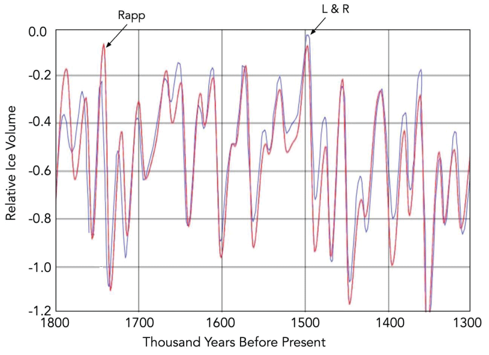
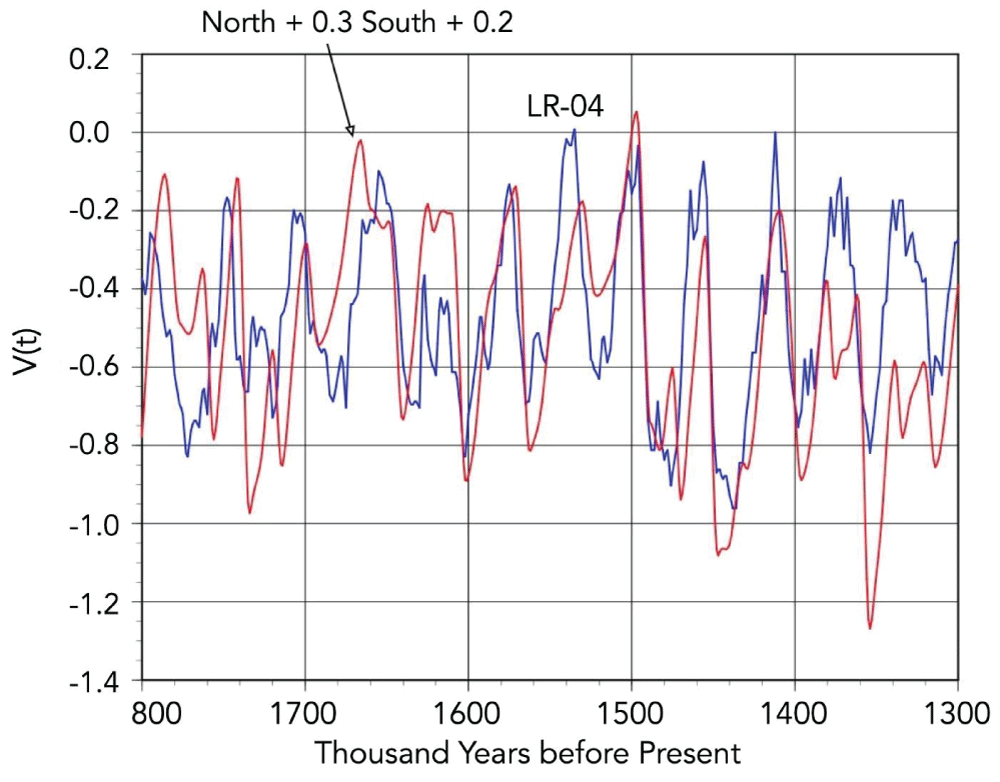
Raymo, et al. (2006) applied the Imbries model to the North and the South in the pre-MPT period. Following Raymo, et al. (2006), I utilized Imbries' equation to model the combination of North ice volume and 0.3 times the calculated South ice volume as shown in Figure 4. That assumes that the maximum change in ice volume in the South was about 30% of the maximum change in ice volume in the North. Note that V(t) is negative. The LR-04 data was scaled to fit on the graph. As Raymo, et al. (2006) pointed out, the agreement of the cadence is remarkable. Despite the fit of the model to the data, this writer remains a bit skeptical. How can Imbries’ model represent reality with its negative V(t), its linear response to a non-linear system, and its gross failure in the post-MPT era? The results seem enigmatic.

Figure 4: Comparison of modeled ice volume vs. time-based on North and South (red curve) to the scaled LR-04 ice volume data (blue curve).

Sophisticated model for the pre-MPT (2023)

Watanabe, et al. (2023) employed a three-dimensional dynamic ice-sheet model to estimate changes in ice volume for a portion of the pre-MPT. [1212Watanabe Y, Abe-Ouchi A, Saito F, et al. Astronomical forcing shaped the timing of early Pleistocene glacial cycles. Commun Earth Environ. 2023;4:113.] They claimed their model provided a good correlation to the observed variation of ice volume (as represented by changes in sea level) from about 1,550 to 1,200 thousand years ago. However, the model is too complex to infer the timing of the cycles in simple terms. The problem with great computer models is that the physics is not evident and it is difficult to ascertain what is forcing the observed changes.

Linkage of North and South

Reference [1313Denton GH, Putnam AE, Russell JL, et al. The Zealandia switch: Ice Age climate shifts viewed from southern moraine. Quat Sci Rev. 2021;257:106771.] is a lengthy paper that deals with several aspects of ice ages. The astronomical theory of ice ages was regarded with some disdain. The main issue considered in this paper is that the entire Earth cooled synchronously in North and South during post-MPT ice ages, yet the solar irradiance in North and South is 180 degrees out of phase. It is also relevant that these authors regarded this as a factor against the astronomical theory of ice ages. However, their reference to the astronomical theory was the single reference [1414Milankovitch M. Kanon der Erdbestrahlung und Seine Andwendung auf das Eiszeirenproblem. Belgrade; 1941.] dated 1941, and they did not refer to any subsequent work such as References [11Rapp D. Ice Ages and Interglacials. Heidelberg: Springer-Praxis Books; 2018.] or [66Muller RA, MacDonald GJ. Ice Ages and Astronomical Causes. London: Springer Publishing Co.; 2002.] that both went far beyond Reference [1414Milankovitch M. Kanon der Erdbestrahlung und Seine Andwendung auf das Eiszeirenproblem. Belgrade; 1941.] to support the astronomical theory. Nor did they refer to the important paper by Raymo, et al. [1111Raymo ME, Lisiecki LE, Nisancioglu KH. Plio-Pleistocene ice volume, Antarctic climate, and the global delta18O record. Science. 2006 Jul 28;313(5786):492-5. doi: 10.1126/science.1123296. Epub 2006 Jun 22. PMID: 16794038.]. They came up with a rather complex theory of ice ages that involves global circulation models, but this appears to this writer to be highly speculative.

Other models

Rapp (2018) provides a review of other models based on the variability of the Sun, volcanism, greenhouse gases, ocean currents, clouds induced by cosmic rays, and models based on the Southern Hemisphere [1515Rapp D. Ice Ages and Interglacials. Heidelberg: Springer-Praxis Books; 2018. Section 7.].

Summary of models

The solar irradiance at high latitudes varies periodically due to variations in precession, obliquity, and eccentricity of the Earth's orbit about the Sun, and the periodicity is dominated by precession with a period of about 21,000 to 22,000 years, whereas variability of global ice volume has much longer periods. Models in which the ice volume is driven by variations in the solar irradiance tend to predict ice volume changing with the period of precession and have difficulty representing the ice volume data. A qualitative picture based on the physics of how ice ages build up and decay in the pre-MPT era and the post-MPT era would be a good starting point for new models. This paper provides such a description.

Materials and methods

In this study, the materials were data on insolation [77Berger WH, Loutre MF. Insolation values for the climate of the last 10 m.y. Quat Sci Rev. 1991;10:297-317.,1212Watanabe Y, Abe-Ouchi A, Saito F, et al. Astronomical forcing shaped the timing of early Pleistocene glacial cycles. Commun Earth Environ. 2023;4:113.], ice volume [1010Lisiecki LE, Raymo ME. A Pliocene-Pleistocene stack of 57 globally distributed benthic δ18O records. Paleoceanography. 2005;20-PA1019.,1212Watanabe Y, Abe-Ouchi A, Saito F, et al. Astronomical forcing shaped the timing of early Pleistocene glacial cycles. Commun Earth Environ. 2023;4:113.], and temperature [22Masson-Delmotte V, Buiron D, Ekaykin A, et al. A comparison of the present and last interglacial periods in six Antarctic ice cores. Clim Past. 2011;7:397-423.] over the past 2 million years. The methods used were tabulating, plotting, inspection, and interpretation of the data, and where appropriate, modeling by integration of differential equations. The purpose was to return to fundamental data and examine the relationships between insolation (SIHL) and ice volume in the pre-MPT and post-MPT eras, to discern the connections between up lobes of SIHL and terminations, and the connections between down lobes in SIHL and starts of ice ages.

The fundamental approach was to compare data year by year over thousands of years, for SIHL and ice volume.

Results

The pre-MPT era

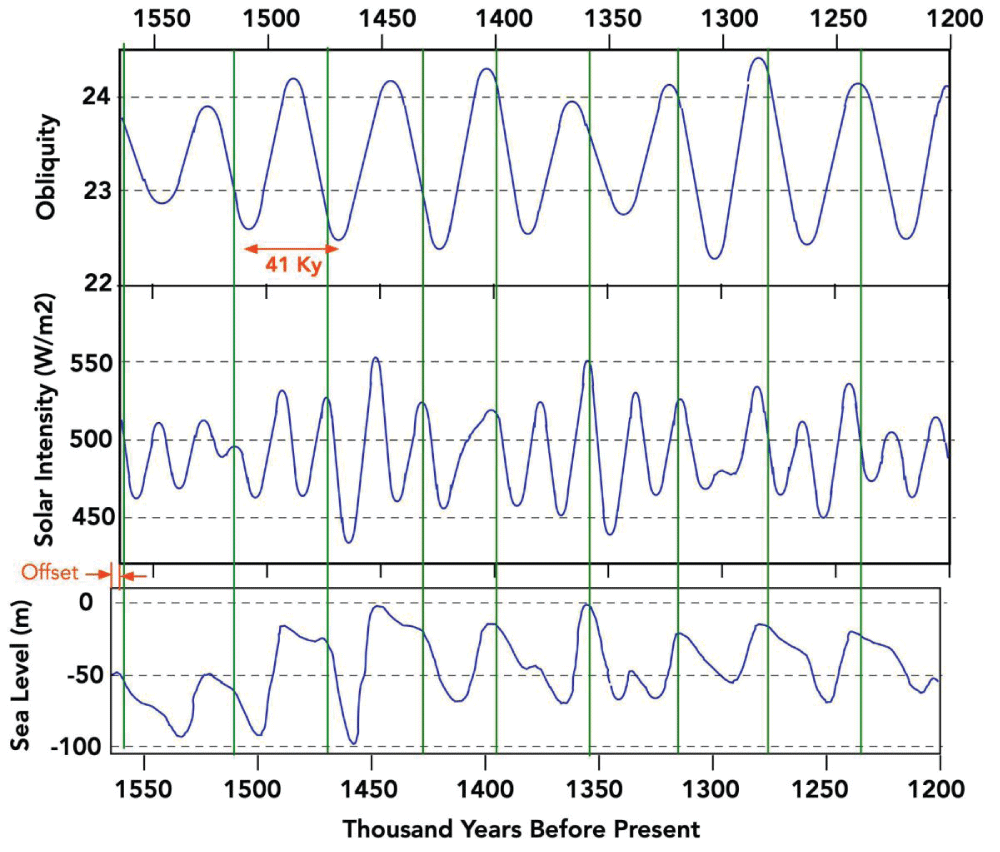
Figure 5 shows a comparison of SIHL, obliquity, and sea level (as an inverse measure of global ice) across a segment of the pre-MPT [1212Watanabe Y, Abe-Ouchi A, Saito F, et al. Astronomical forcing shaped the timing of early Pleistocene glacial cycles. Commun Earth Environ. 2023;4:113.]. This figure shows that sharp drops in sea level (increases in ice volume) occur only at SIHL down lobes. However, not all SIHL down lobes cause a drop in sea level. Furthermore, the SIHL down lobes that produce a drop in sea level are not always the down lobes with the greatest amplitude.

1212Watanabe Y, Abe-Ouchi A, Saito F, et al. Astronomical forcing shaped the timing of early Pleistocene glacial cycles. Commun Earth Environ. 2023;4:113.]." /> Figure 5: Obliquity, solar power, and sea level in a segment of the pre-MPT era. Green lines show onsets of ice ages. Data from Watanabe, et al. (2023) [1212Watanabe Y, Abe-Ouchi A, Saito F, et al. Astronomical forcing shaped the timing of early Pleistocene glacial cycles. Commun Earth Environ. 2023;4:113.].

The power absorbed by the surface depends on the product of insolation (SIHL) and the absorptivity of the surface. The absorptivity is greater, the closer the solar rays are to the normal surface. The greater the obliquity, the greater the angle between the solar rays and the normal to the surface, so the absorptivity is less at higher obliquity.

It can be seen in Figure 5 that when the obliquity down lobe occurs in the same time regime as a solar down lobe – the sea level drops sharply indicating the beginning of an ice age (see vertical green lines). These occurrences appear to be spaced roughly regularly at approximately 41,000-year intervals (same as spacing of obliquity). There is an approximate resonance between the 41,000-year spacing of variations of obliquity and the 21,000-22,000-year spacing of precession so that almost every other precession down lobe occurs when there is an obliquity down lobe, resulting in minimum power absorbed by the surface, inducing glaciation. The data indicates that the start of an ice age requires solar and obliquity down lobes to occur in the same time regime. To get the best fit, the solar curves were shifted to the right for a few thousand years. This might be due to a time lag between changes in solar and changes in ice volume, or possibly the sea level time scale is off, or some combination of the two.

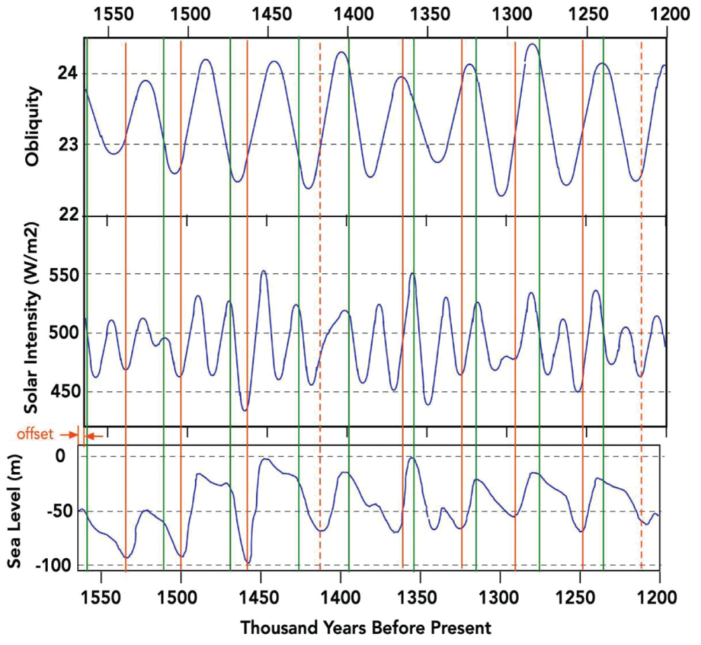
Figure 6 shows a comparison of SIHL, obliquity, and sea level (as an inverse measure of global ice) across a segment of the pre-MPT [1212Watanabe Y, Abe-Ouchi A, Saito F, et al. Astronomical forcing shaped the timing of early Pleistocene glacial cycles. Commun Earth Environ. 2023;4:113.]. This figure shows that sharp increases in sea level (decreases in ice volume) occur only at SIHL up lobes. However, not all SIHL up lobes cause a rise in sea level. Furthermore, the up lobes in SIHL that produce an increase in sea level are not always the up lobes with the greatest amplitude. The green lines show the start of the ice age, and the red lines show the termination of ice age. Dashed lines show fewer changes than solid lines.

1212Watanabe Y, Abe-Ouchi A, Saito F, et al. Astronomical forcing shaped the timing of early Pleistocene glacial cycles. Commun Earth Environ. 2023;4:113.]." /> Figure 6: Obliquity, solar power, and sea level in a segment of the pre-MPT era. Green lines show onsets of ice ages and red lines show terminations of ice ages. Data from Watanabe, et al. (2023) [1212Watanabe Y, Abe-Ouchi A, Saito F, et al. Astronomical forcing shaped the timing of early Pleistocene glacial cycles. Commun Earth Environ. 2023;4:113.].

We conclude that approximately every 41,000 years, the obliquity and SIHL undergo down lobes in the same time regimes, resulting in an ice age building up over very roughly 10,000 years. As time progresses, SIHL and obliquity run out of phase and the ice volume decreases slightly but the ice age remains. Finally, very roughly 20,000 years after the start of the ice age, the obliquity and SIHL both enter the same time regimes and up lobes bringing about the start of a termination of the ice age. The ensuing interglacial lasted roughly 10,000 years. This cycle repeats itself with roughly 30,000-year ice ages and very roughly 10,000-year interglacials. The ice ages appear to be very roughly 41,000 years apart. The exact timing varies from these round numbers from occasion to occasion.

The post-MPT era

Post-MPT data: In the post-MPT era, the Earth was colder than it was in the pre-MPT era, and the ice sheets were more extensive and more robust, once started, they reached sufficient extent that they were better able to withstand up lobes in SIHL that occurred afterward. The ice age cycles were quite different from those in the pre-MPT period, yet the variation of the solar parameters was essentially the same.

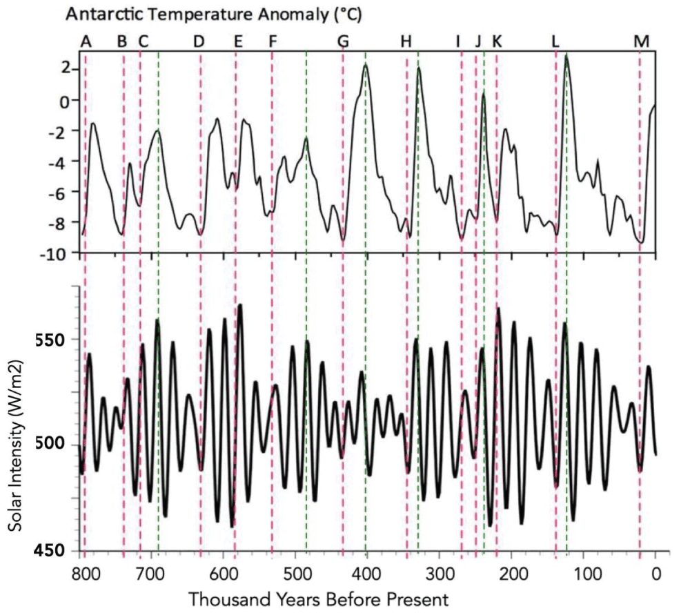
Figure 7 shows a comparison of the SIHL to the Antarctic temperature anomaly in the post-MPT era [1616Rapp D. Ice Ages and Interglacials. Heidelberg: Springer-Praxis Books; 2018. Section 8.6.4.]. Each start of a major ice age (green dashed lines) occurs as an SIHL down lobe begins. All the sharp temperature increases (terminations – red dashed lines) occur as an SIHL up lobe begins.

1616Rapp D. Ice Ages and Interglacials. Heidelberg: Springer-Praxis Books; 2018. Section 8.6.4.]." /> Figure 7: Comparison of Antarctic temperature (from ice cores) to variations in SIHL. The red dashed lines show onsets of termination of ice ages at solar up lobes. The green dashed lines show the onset of glaciation at solar down lobes [1616Rapp D. Ice Ages and Interglacials. Heidelberg: Springer-Praxis Books; 2018. Section 8.6.4.].

Not every SIHL down lobe produces glaciation. Not every SIHL up lobe produces a termination. Why?

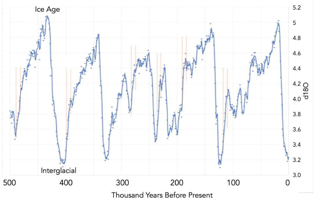
The ocean sediment data for δ¹⁸O (which is a measure of global ice volume) over the last 500,000 years is shown in Figure 8. The faint red lines show that a large expansion of ice takes place in the first down lobe of SIHL, spreading ice so far that the next up lobe in SIHL cannot terminate the ice age, but only slows its growth temporarily. The ice age continues to expand with further accumulation of ice for typically 4 or 5 cycles of precession. Eventually, rapid termination occurs at the down lobe of SIHL.

11Rapp D. Ice Ages and Interglacials. Heidelberg: Springer-Praxis Books; 2018.]." /> Figure 8: 18O as measured by ocean sediments in the last 500,000 years. The rapid spread of ice in the initial several thousand years is emphasized by faint vertical red lines [11Rapp D. Ice Ages and Interglacials. Heidelberg: Springer-Praxis Books; 2018.].

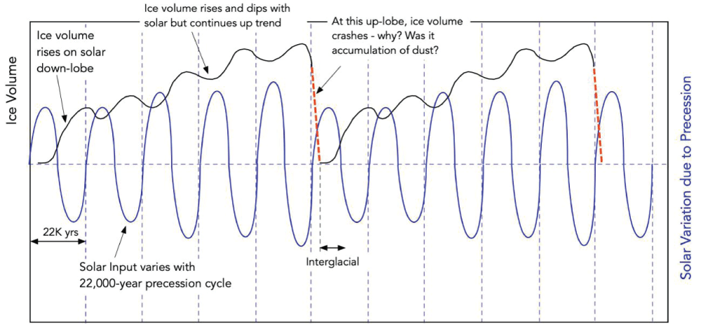
Model for post-MPT: The post-MPT data tells us that coming out of an interglacial, ice age starts at the next down lobe of SIHL. Once an ice age starts in the post-MPT era, the extent of glaciation expands rapidly over several thousand years. Each successive down lobe of SIHL adds to the ice volume and each successive up lobe of SIHL temporarily slows down ice accumulation but does not necessarily terminate the ice age. The ice volume continues to grow until a particular up lobe of SIHL brings about a termination. This is illustrated schematically in Figure 9.

Figure 9: Model for ice ages in the post-MPT era.

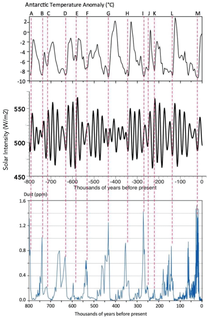
The question is why does termination occur at this up lobe of SIHL? The answer might be that accumulation of dust on the ice late in an ice age increases its absorptivity and when that builds up sufficiently, the next-up lobe in SIHL brings about a termination. Figure 10 shows that the major terminations late in the post-MPT era all occurred at SIHL up lobes accompanied by high dust levels.

11Rapp D. Ice Ages and Interglacials. Heidelberg: Springer-Praxis Books; 2018.,1717Ellis R, Palmer M. Modulation of ice ages via precession and dust-albedo feedbacks. Geosci Front. 2016. Available from: http://www.sciencedirect.com/science/article/pii/S1674987116300305]." /> Figure 10: Dust levels at an overlapping time scale as SIHL and temperature in Antarctic ice cores [11Rapp D. Ice Ages and Interglacials. Heidelberg: Springer-Praxis Books; 2018.,1717Ellis R, Palmer M. Modulation of ice ages via precession and dust-albedo feedbacks. Geosci Front. 2016. Available from: http://www.sciencedirect.com/science/article/pii/S1674987116300305].

Ellis and Palmer (2016) provided extensive evidence that the deposition of dust on the ice sheets provided a decrease in ice-albedo that acted as a trigger to enable the next precession up-lobe to melt the ice sheets [1717Ellis R, Palmer M. Modulation of ice ages via precession and dust-albedo feedbacks. Geosci Front. 2016. Available from: http://www.sciencedirect.com/science/article/pii/S1674987116300305]. Only at the depth of an ice age (at the lowest temperature and the lowest CO₂ concentration) after 4 or 5 precession cycles had evolved, would sufficient dust be deposited on the ice sheets to cause albedo reductions and glacial termination. There is good evidence that Antarctic dust levels peaked before each termination, but we only have Arctic dust data for the last termination. However since this limited Arctic dust data agrees so well with the Antarctic dust record, it is not unreasonable to assume that Arctic dust flux was closely correlated with Antarctic dust since the MPT. It seems likely that the effects of SIHL variations were being masked by the albedo-feedback-driven tendency toward glaciation in the North, until dust deposition decreased the albedo, thus allowing an SIHL up-lobe to produce a termination. The pattern during the period from 800,000 years ago to 450,000 years ago was not as regular as that after 450,000 years ago, but the spacing of major glacial-interglacial periods tended to be very roughly four precessional cycles. The data for the past five ice ages indicate that the heat balance of higher northern latitudes favored glaciation, and lacking any unusual internal Earth factor, the ice sheets at higher northern latitudes would have continued to grow unabated. The data indicate that precessional up-lobes in SIHL in the North might have produced temporary slowdowns in the expansion of the ice sheets, but the long-term trend through at least four precessional periods was a continuing expansion of the ice sheets. The data also show that after 4 or 5 precessional cycles, the growth of the ice sheets came to a rather sudden halt, and a termination ensued in which the ice sheets melted in roughly 7,000 years.

We surmise from the work of Peltoniemi, et al. (2015) that solar elevation is a crucial parameter for bringing about a glacial termination resulting in an interglacial [1818Peltoniemi JI, Gritsevich M, Hakala T, et al. Soot on snow experiment: Bidirectional reflectance factor measurements of contaminated snow. The Cryosphere. 2015;9:2323-2337.]. The solar elevation at solar noon at mid-summer is {90° – (latitude) + (obliquity)}. At 65°N latitude, the solar elevation at solar noon at mid-summer is {25° + (obliquity)}. As the obliquity ranges from about 22° to 24°, the sine of the solar elevation at solar noon at mid-summer ranges from 0.258 to 0.269, an increase of 4%.

These observations lend some credence to the idea that terminations originate at a precessional upswing in SIHL immediately after major dust deposition.

Discussion

There is little doubt that oscillations in SIHL, induced by variations in the Earth’s orbit, are the main drivers for the recurrent cycles of glacial and interglacial periods. Spectral analysis demonstrates the participation of the orbital parameters [11Rapp D. Ice Ages and Interglacials. Heidelberg: Springer-Praxis Books; 2018.,66Muller RA, MacDonald GJ. Ice Ages and Astronomical Causes. London: Springer Publishing Co.; 2002.].We have demonstrated here that essentially all terminations of ice ages occur on up lobes of SIHL, while ice ages begin on down lobes of SIHL. The big questions are why some up lobes produce terminations while others do not, and why some down lobes originate ice ages while others do not. The answer to these questions is subdivided into pre-MPT and post-MPT eras.

In the pre-MPT era, we find that ice ages originate at periods when the SIHL is entering a down lobe and the obliquity is minimal, resulting in a combination of low SIHL and higher reflectivity (at lower obliquity which makes the solar angle at high latitude more glancing). Ice ages terminate at a coincidence of high SIHL and high obliquity. Because the timing of variations in obliquity is almost double that of precession, the occurrence of these links between SIHL and obliquity tends to be repetitive with approximately 41,000-year spacing.

In the post-MPT era, we find that ice ages also originate at a down lobe of SIHL. Because the Earth is now cooler than in the pre-MPT era, once an ice age is started, there is a rapid increase in the spread of ice, so that each successive up lobe in SIHL might cause a slight decrease in ice volume but is unable to bring about a termination. Each down lobe that follows adds to the ice volume. The ice age continues to expand as up-lobes and down-lobes of SIHL continue to occur. After several precession cycles, the effect of global cooling creates a very dusty atmosphere, and when high dust levels and an up lobe become coincident in time, a termination occurs.

This paper is qualitative. To solidify the qualitative conclusions in this paper, one would have to carry out quantitative estimates of the proposed effects that influence the start or end of ice ages. That includes the dependence of energy absorbed on the average angle of solar rays to the surface, and the dependence of energy absorbed on the amount of dust deposited on ice sheets.

Conclusion

The astronomical theory of ice ages is widely accepted. Periodic changes in key parameters of the Earth’s orbit produce variations in the Solar Input to High Latitudes (SIHL) and ice ages begin on down lobes of SIHL and terminate on up lobes of SIHL. However, not all down lobes create ice ages and not all up lobes produce terminations. The ice ages changed character at the so-called mid-Pleistocene transition, about a million years ago. The actual amount of power absorbed by the surface depends on SIHL and the absorptivity of the surface. The absorptivity is affected by the obliquity in the pre-MPT era, and by dust deposits late in the post-MPT era. When these are included, we can rationalize why some down lobes produce ice ages, and some up lobes produce terminations in both eras.

In the pre-MPT era, ice ages originate when the SIHL enters a down lobe and the obliquity is minimal (higher reflectivity) and ice ages terminate at a coincidence of high SIHL and high obliquity. These links between SIHL and obliquity tend to be repetitive with approximately 41,000-year spacing.

In the post-MPT era, ice ages originate at a down lobe of SIHL. Once an ice age is started, each successive up lobe in SIHL might cause a slight decrease in ice volume but doesn’t bring about a termination. After several precession cycles, high dust levels increase absorptivity, and the next-up lobe produces a termination.

The uncertainty in the connection between variations in SIHL and variations in global ice volume is now resolved.

Author contributions: Donald Rapp carried out the entire study.

Highlights

It is widely accepted that variations in insolation to high latitudes are the driving force for the observed periodic occurrence and termination of ice ages. This paper provides rationalizations for why some increases in insolation to high northern latitudes produce terminations and some do not, and why some decreases in insolation to high northern latitudes induce ice ages, and some do not. It also provides a rationale for why the spacing of ice ages changes across the Mid-Pleistocene Transition (MPT).

References

1. Rapp D. Ice Ages and Interglacials. Heidelberg: Springer-Praxis Books; 2018.

2. Masson-Delmotte V, Buiron D, Ekaykin A, et al. A comparison of the present and last interglacial periods in six Antarctic ice cores. Clim Past. 2011;7:397-423.

3. Rapp D. Ice Ages and Interglacials. Heidelberg: Springer-Praxis Books; 2018. Section 1.

4. Rapp D. Ice Ages and Interglacials. Heidelberg: Springer-Praxis Books; 2018. Section 6.

5. Rapp D. Ice Ages and Interglacials. Heidelberg: Springer-Praxis Books; 2018. Section 9.2.

6. Muller RA, MacDonald GJ. Ice Ages and Astronomical Causes. London: Springer Publishing Co.; 2002.

7. Berger WH, Loutre MF. Insolation values for the climate of the last 10 m.y. Quat Sci Rev. 1991;10:297-317.

8. Imbrie J, Imbrie JZ. Modeling the climatic response to orbital variations. Science. 1980;207:943-953.

9. Paillard D. The timing of Pleistocene glaciations from a simple multiple-state climate model. Nature. 1998;391:378-381.

10. Lisiecki LE, Raymo ME. A Pliocene-Pleistocene stack of 57 globally distributed benthic δ18O records. Paleoceanography. 2005;20-PA1019.

11. Raymo ME, Lisiecki LE, Nisancioglu KH. Plio-Pleistocene ice volume, Antarctic climate, and the global delta18O record. Science. 2006 Jul 28;313(5786):492-5. doi: 10.1126/science.1123296. Epub 2006 Jun 22. PMID: 16794038.

12. Watanabe Y, Abe-Ouchi A, Saito F, et al. Astronomical forcing shaped the timing of early Pleistocene glacial cycles. Commun Earth Environ. 2023;4:113.

13. Denton GH, Putnam AE, Russell JL, et al. The Zealandia switch: Ice Age climate shifts viewed from southern moraine. Quat Sci Rev. 2021;257:106771.

14. Milankovitch M. Kanon der Erdbestrahlung und Seine Andwendung auf das Eiszeirenproblem. Belgrade; 1941.

15. Rapp D. Ice Ages and Interglacials. Heidelberg: Springer-Praxis Books; 2018. Section 7.

16. Rapp D. Ice Ages and Interglacials. Heidelberg: Springer-Praxis Books; 2018. Section 8.6.4.

17. Ellis R, Palmer M. Modulation of ice ages via precession and dust-albedo feedbacks. Geosci Front. 2016. Available from: http://www.sciencedirect.com/science/article/pii/S1674987116300305

18. Peltoniemi JI, Gritsevich M, Hakala T, et al. Soot on snow experiment: Bidirectional reflectance factor measurements of contaminated snow. The Cryosphere. 2015;9:2323-2337.

記事について

この記事を引用する

Rapp D. Revisiting Ice Ages Cycles. August 22, 2024; 2(8): 726-733. IgMin ID: igmin239; DOI: 10.61927/igmin239; Available at: igmin.link/p239

• DOI10.61927/igmin239

08 Aug, 2024

受け取った

21 Aug, 2024

受け入れられた

22 Aug, 2024

発行された

この記事を共有する

次のリンクを共有した人は、このコンテンツを読むことができます:

共有リンクを取得する

トピックス

Earth Science