The Influence of Dynamical Downscaling and Boundary Layer Selection on Egypt’s Potential Evapotranspiration using a Calibrated Version of the Hargreaves-samani Equation: RegCM4 Approach

Abstract

Potential Evapotranspiration (PET) is an important variable for monitoring daily agricultural activity as well as meteorological drought. Therefore, it is necessary to investigate the influence of different options of the physical dynamical downscaling and boundary layer schemes on the simulated PET. Using the RegCM4 regional climate model, four simulations were conducted (two for each case) in the period 1997 to 2017. In all simulations, the RegCM4 was configured with 25 km resolution and downscaled by the ERA-Interim reanalysis dataset. To ensure a reliable estimation of the PET, a calibrated version of the Hargreaves-Samani equation was adopted. A high-resolution product of the ERA5 was used as the observational dataset. Results showed that the simulated PET is iNSEnsitive either to the dynamical downscaling or the boundary layer options. Concerning the annual climatological cycle, the RegCM4’s performance varies with month and location. Quantitatively, a root mean square error lies between 1 mm and 1.6 mm day^-1, the Nash-Sutcliffe efficiency between 0.2 and 0.6, and the coefficient of determination between 0.5 and 0.75. Additionally, the Linear Scaling (LS) method showed its added value in the evaluation/validation periods. In conclusion, the RegCM4 can be used to develop a regional PET map of Egypt using the LS either in the present climate or under different future scenarios.

Introduction

The Middle East and Northern Africa (MENA), a region known for having limited water resources, has more significant water needs, as stated in the Assessment Report by the Intergovernmental Panel on Climate Change [1,2]. Total evapotranspiration, a measure of demand, has increased due to rising mean air temperatures. This trend is particularly pronounced under different future scenarios [3,4]. There are four critical components to comprehending total evapotranspiration: i) Potential evapotranspiration (PET), ii) reference evapotranspiration, iii) crop evapotranspiration, and iv) Actual evapotranspiration are the four categories. In this context, our focus is on potential evapotranspiration (PET). Allen, et al. [5] define PET as the greatest rate of evaporation feasible under the current meteorological conditions, regardless of soil moisture levels.

The relevance of PET is made clear by how it affects desert zone agriculture and water resources. In areas where water is scarce, changes in PET are especially significant. In addition, PET controls how severe a drought is in desert regions [6]. The Penman-Monteith equation (PM; [7]), which is recommended for the PET estimate because it is based on fundamental ideas guiding the movement of energy and water between the earth’s surface and the atmosphere, calls for a wide range of atmospheric variables. Sperna Weiland, et al. [8] and Murat, et al. [9] reported that a significant increase in the uncertainty related to estimated PET is caused by many of these variables being generated empirically. As a result, several approaches for estimating PET have been developed globally to solve this problem, each one being specific to the availability of input factors in a given region.

The Hargreaves-samani equation (HS; [10]) has become one of the most often used approaches for overcoming these difficulties as a result of its simplicity and use [11-13]. It is noteworthy that the HS equation uses the mean air temperature as its single input variable [14], a quantity that is easily measured and frequently recorded in meteorological records. The Penman-Monteith equation (PM) can be replaced by the HS equation, which is derived from the relationship between air temperature and potential evapotranspiration (PET), particularly in regions with sparse access to extensive weather data [15,16]. Another notable benefit of the HS equation is its ability to forecast future PET changes under various climatic scenarios [17,18]. The mean air temperature, a quantity easily retrieved from meteorological databases, provides the basis for this projection. Anticipating forthcoming alterations in PET holds paramount importance for regions encompassing a wide range of hydro-climatic conditions (e.g., [19]). Planning for agriculture, hydrological modeling, and the investigation of meteorological droughts are all made possible by it [20-22]. The HS equation emerges as a useful tool when taking into account the critical necessity to comprehend the potential implications of climate change on PET for adjusting to changing environmental dynamics [23-25].

High-Resolution Regional Climate Models (RCMs) must be used to create reliable regional maps of Potential Evapotranspiration (PET) for both the present and the future climates [26-28]. Temperature, humidity, wind speed, and solar radiation are all important factors in PET simulations, and these models provide a thorough examination of a variety of climatic parameters [5]. In addition to providing a high spatial resolution, improving the precision of PET estimates necessitates looking into various options for dynamical downscaling and utilizing physical procedures (raising the accuracy of PET estimation). RCMs are essential for replicating extremely accurate topographical data and capturing localized weather patterns with better fidelity in dynamic downscaling [29]. Additionally, boundary layer schemes must be taken into account to improve the accuracy of atmospheric variables used in PET calculations. These schemes contribute to a more nuanced understanding of atmospheric processes, thus bolstering the accuracy of PET estimates.

Xu, et al. [30] highlighted that large-scale atmospheric circulations can be successfully replicated with enhanced physical parameterization and high-resolution Regional Climate Models (RCMs). They ran several simulations with the RegCM4 model, considering various reanalysis outputs, to constrain mean air temperature and total surface precipitation. They found that using a one-way nesting approach does not guarantee greater performance than straight downscaling to high resolution. To assess the effectiveness of direct downscaling (interpolating the global low-resolution general circulation model to the high-resolution spacing provided by the regional climate model) and one-way nesting [involves two steps: 1 - interpolating the global low-resolution general circulation model to a coarse-resolution spacing (e.g. 75 km) provided by the regional climate model and 2 – the coarse-resolution domain provides the lateral boundary condition to the high-resolution grid spacing domain] for the daily mean air temperature, Anwar [31] applied the RegCM4 in Egypt. It was found that direct downscaling yielded better results than one-way nesting, which is consistent with the findings reported by [30]. This study highlights how important it is to select a suitable downscaling method for precise climate modeling and prediction.

Using RegCM4, the role of physical parameterization has been investigated in various applications in Egypt. For instance, Ali, et al. [32] investigated the role of boundary layer parameterization in exploring the dynamical features of a dust storm using the RegCM4. They found that the HOLTSLAG (HOLT; [33]) is the best scheme to simulate the dust storm dynamics concerning reanalysis products and in-situ observations. Concerning the surface climate, Anwar and Mostafa [34] used RegCM4 to investigate how boundary layer designs affected Egypt’s daily mean air temperature. The two boundary layer schemes are the University of Washington (UW; [35]) and HOLTSLAG. They observed that the UW scheme outperforms the HOLT scheme in simulating mean air temperature. Furthermore, it has been reported that neither the boundary layer schemes (HOLT or UW; [34]) nor the downscaling methodology (direct or one-way nesting; [31]) had an impact on global incident solar radiation. This suggests that these configurations might not have a substantial impact on incoming solar radiation globally and emphasizes the value of precise boundary layer models in forecasting the daily mean air temperature.

Anwar and Lazic [36] investigated the added value of calibrating the HS equation as well as the influence of the lateral boundary condition that drives the RegCM4 model to recreate the ERA5 dataset. However, they didn’t consider the role of different options of the dynamical downscaling and boundary layer schemes in simulating the PET. Therefore, the present study aims to explore the possible influence of such options as well as the added value of applying the bias-correction method of linear scaling (LS; [37]). The main goal is to reduce the bias of RegCM4 across different periods and grid locations. Our paper is organized as follows: section 2 describes the study area and experiment design; Section 3 shows the results of the study. Section 4 provides the discussion and section 5 shows the conclusion and future work.

Materials and methods

Study area

Egypt (an important country in the MENA region) is bounded by the Mediterranean Sea from the north and the Red Sea from the east. From a climatic point of view, Egypt is categorized as semi-arid, with minimal precipitation ([38,39]. Concerning the wind regime, Egypt is characterized by a particular regime along the Red Sea and Mediterranean shores. According to the Köppen climate classification [40], Egypt is classified as a hot desert climate (BWh). Also, Egypt receives between 20 mm and 200 mm of annual average precipitation along the Mediterranean coast. Concerning relative humidity, the maximum and annual values vary with the region of study. For instance, Cairo has minimum values during spring (around 48%) and maximum values in summer (around 70%). In addition, Egypt is characterized by heatwaves during the spring and summer seasons (inteNSE in Upper Egypt and moderate in the Northern Coast). Concerning the coast of the Mediterranean Sea, the dominant wind direction is northwest, which can explain the moderate temperature along the Mediterranean coast. However, the situation is different in the central and the southern sectors because nighttime temperatures are very hot, especially in the summer, when average high temperatures can exceed 40 °C, as in Aswan, Luxor, Asyut, or Sohag. Additionally, the high-elevation topography (e.g., Saint Catherine Mountains) plays an important role in cooling the nighttime temperature.

Experiment design

The Regional Climate Model (RegCM) of the International Center of Theoretical Physics was used in the present study. The RegCM was developed at the National Center for Atmospheric Research (NCAR, [41,42]). The RegCM is an open-source model, and it is used for various applications, such as regional process studies, paleoclimate simulations, future climate projections, chemistry-climate interactions, aerosol effects, and biosphere-atmosphere interactions [43]. Also, RegCM passed through a series of developments from RegCM1 [42], RegCM2 [44,45], RegCM3 [46] and RegCM4 [47]. Recently, a new version of the RegCM has been developed and tested (RegCM5; [48]). During the time of the study, a stable version of the RegCM5 was not available. Instead, we used version 4.7 of the RegCM (hereafter RegCM4). Concerning PET, RegCM4 has been used to compute the PET in different regions such as Egypt [18,36], Bulgaria [49], and Tropical Africa [50]. To address the influence of different options of dynamical downscaling and boundary layer schemes on the simulated PET, four experiments were conducted over the period 1997–2017. The first year was considered as a spin-up to initialize the RegCM4 model with an equilibrium state of the atmosphere as recommended by [51,52], so the actual analysis starts in 1998 and ends in 2017. It is important to mention that the effect of aerosols was not included in the present study.

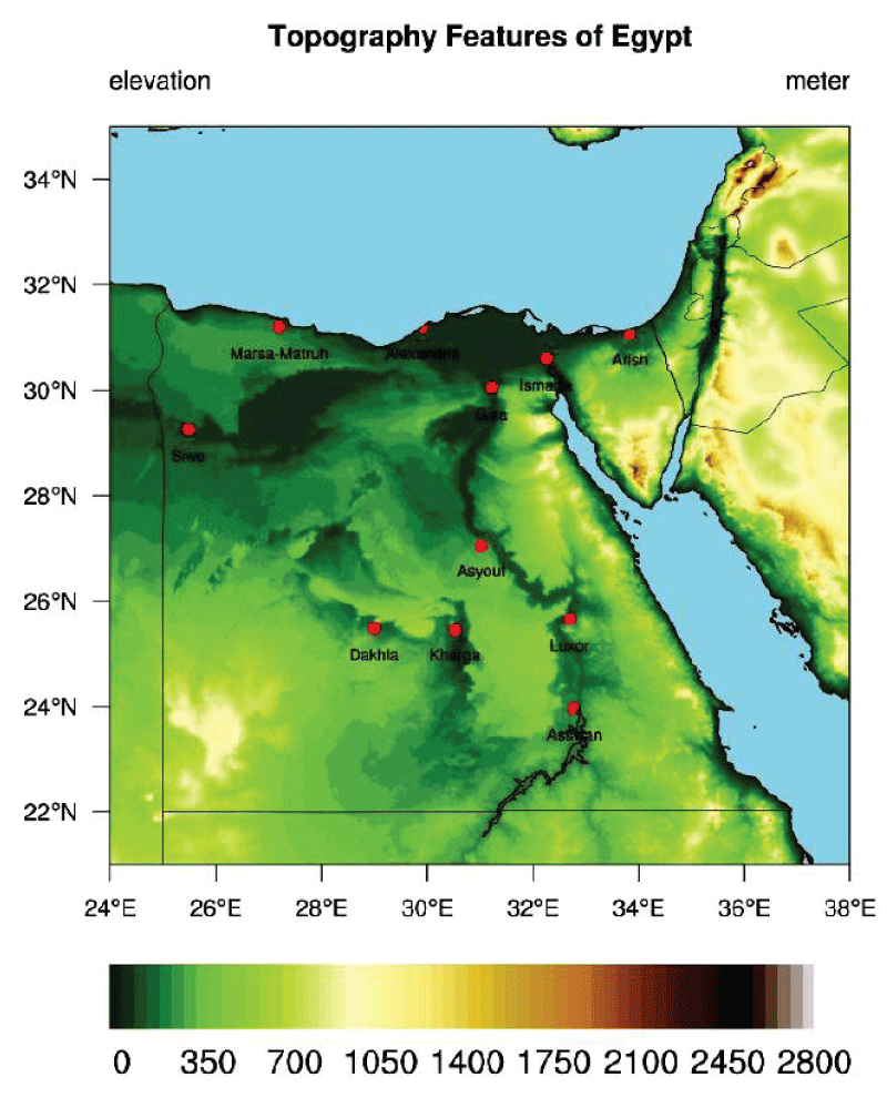
In the present study, the RegCM4’s domain was customized with 25 km horizontal resolution with 60 grid points in both zonal and meridional directions centered at latitude 27 °N and longitude 30 °N. The RegCM4 was used to downscale the ERA-Interim reanalysis of 1.5 degrees (EIN15; [53]) to provide the lateral boundary condition and sea surface temperature. Figure 1 shows the surface elevation of Egypt (in meters) including the locations reported in [18]. To serve the purpose of the present study, the four simulations were grouped into two cases. The first case considers the dynamical downscaling options: direct (DIR) and one-way nesting (NEST) following [31]. On the other hand, the second case manipulates the boundary layer scheme: HOLT and UW following [34]. The PET was calculated using a calibrated version of the HS equation following [36] in the four simulations. The model domain and physical configurations are summarized in Table 1. The calibrated HS equation is written as:

$PE{T}_{HS}=0.0105 \times RSDS\times (TMP+ 17.8)$ (1)

where RSDS is the global incident solar radiation (expressed in mm day^-1 to match the PET unit; [5]) and TMP is the 2 m mean air temperature (in °C). PET is the potential evapotranspiration (in mm day^-1). In each case, the simulated PET was evaluated for the derived ERA5-land reanalysis product [54]. In addition, the significant difference between the two simulations (in each case) was calculated using the student t-test with alpha equals 5%. Following [49], the following statistical metrics were used to quantify the simulated PET (on a point scale) concerning the ERA5 concerning the climatological annual cycle: coefficient of determination (R²), Nash-Sutcliffe efficiency (NSE) and a root mean square error (RMSE).

$R^2= {(\frac{N{\displaystyle \sum S_{i }{R}_{i }}- {\displaystyle \sum S_i} {{\displaystyle {\displaystyle \sum R_i}}}^{\text{}}}{\sqrt{N {{\displaystyle {\displaystyle \sum S_i^2}}}^{\text{}}-{\displaystyle \sum s_i^2} } \sqrt{N {{\displaystyle {\displaystyle \sum R_i^2}}}^{\text{}}- {\displaystyle \sum R{s}_i^2} }})}^2$ (2)

$NSE=1-\frac{{\displaystyle {\sum }_1^N{{\displaystyle {(S_i- R_i)}^2}}_{}^{}}}{{{\displaystyle {\displaystyle {\sum }_1^N{(R_i- {\overline{R}}_i)}^2}}}_{}^{}}$ (3)

$RMSE= \sqrt{\frac{1}{N} {\displaystyle \sum }_1^N{(\stackrel{-}{S_i}- \stackrel{-}{R_i})}^2}$ (4)

where N represents the total number of records for both the RegCM4 and ERA5, ${\dot{S}}_{\text{i }}$ and ${\dot{R}}_{\text{i }}$ represents the average of RegCM4 and ERA5 for each month i, respectively. To possibly reduce the simulated PET bias, the LS bias-correction technique was used. In Egypt, the LS provided its efficiency in bias reduction concerning the observed data [55,56]. Nashwan, et al. [55] applied the LS method for each grid point, while Mostafa, et al. [56] used the LS for a point scale. Also, in the aforementioned studies, the climatological bias was corrected for each month. In the present study, the climatological bias was calculated for each season. In this case, the LS method can be written as:

$PE{T}_{new,(i)}= PE{T}_{(i)}+ \left(OB{S}_{clim,\left(i\right)}- PE{T}_{clim,\left(i\right)}\right),$ (5)

where PETi is the simulated PET (of each season) before applying the LS, PET_new,(i) is the simulated PET after considering the LS method. OBS_clim,(i) and PET_clim,(i) are the climatological averages of the observed and simulated PET of each season respectively. To validate the LS method, two steps were followed:

The period 1998 – 2017 was divided into two segments: 1998 – 2008 as the evaluation period and 2009 – 2017 as the validation period.

The climatological bias (of each season) in the period 1998 – 2008 was added to each season of the period 2009 – 2017.

Please note that the climatological bias (for each season) was calculated for each grid point using the Climate Data Operator (CDO; https://code.mpimet.mpg.de/projects/cdo/). Also, figures of the PET seasonal climatology were visualized using the NCAR Command Language (NCL; https://www.ncl.ucar.edu/). The time series (for the locations indicated in Figure 1) was extracted from the RegCM4 output using the netCDF Operator (NCO; https://nco.sourceforge.net/) and the bilinear interpolation method.

Figure 1: The figure shows the surface elevation of Egypt (in meters). The red dots indicate the location of the ten locations for evaluating the RegCM’s performance.

Validation data

Long-term recordings of the PET station data in Egypt were not available during the time of study, either spatially or temporally. However, there has recently been the development of a new high-resolution gridded PET reanalysis product (hPET; [54]). This product retrieves the meteorological data (used in computing the PET) from the ERA5-land product and computes the PET using the PM equation. The hPET product is available at 0.1 degrees for a duration of 42 years (1981 – 2023) on an hourly timescale as well as the daily sum. Singer, et al. [54] reported that hPET shows good consistency with available global PET products, particularly the Climate Research Unit (CRU; [58]). The ERA5-Land provides meteorological and land surface variables using the offline land surface model of the ERA5 in a high grid spacing (0.1 degrees; [57]) over the period 1950 to 2023. In addition, it provides accurate estimates of the aforementioned variables because it combines model data and in-situ observations across the world. It is important to mention that the ERA5-Land dataset possesses sources of uncertainty, such as 1 - insufficient representation of some physical processes governing the climate system and 2 – lack of in-situ observations in the region of study. However, the ERA5-land can provide useful information to decision-makers because of its temporal and spatial resolution.

To calculate the PET from the ERA5-land (hoped), the following meteorological variables were needed: 10 m u-component (zonal) of wind speed (m s^-1), 10 m v-component (meridional) of wind speed (m s^-1), 2 m dew point temperature (K), 2 m air temperature (K), surface net solar radiation (J m^-2), surface net thermal radiation (J m^-2) and atmospheric surface pressure (Pa). The hPET is calculated on an hourly timescale for each grid point using the PM equation [7]. To avoid linking it to specific conditions of the vegetated surface or soil moisture conditions, the term PET was considered to calculate the total evapotranspiration. The reader can refer to [54] for additional details concerning the calculation of the hPET.

Besides, hPET products can be used in various topics such as ecohydrology, and drought propagation. Additional advantages of hPET can be found in [58]. Recently, hPET was used to assess the RegCM4 model performance concerning the original and the calibrated version of the HS equation [36]. For the present study, hPET was bilinearly interpolated on the RegCM4 curvilinear grid as recommended by [56]. For evaluation of the RegCM4 on a point scale, all locations (reported in [18]) were considered except for Port-Said and Marsa-Matruh because ERA5 data give missing records in those locations. It is important to mention that the hPET was considered as the observational dataset over the CRU for various reasons such as 1 – hPET is available at 0.1 degrees while the PET is available at 0.5 degrees, 2 – hPET is a reanalysis product (combines the advantages of the model parameterization and in-situ observations), while the CRU is mainly based on upscaling of the meteorological stations across the globe and 3 – the CRU is only available on monthly timescale and hPET is available on a hierarchy of time scales ranging from hourly to monthly.

Results

Seasonal climatology

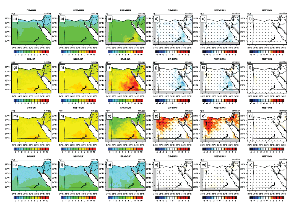
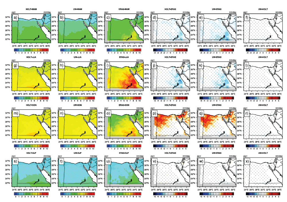
Influence of dynamical downscaling options on PET: Figure 2 explores the influence of dynamical downscaling options (DIR and NEST) on the simulated PET concerning the ERA5 reanalysis product as well as the difference between NEST and DIR. In general, it can be noted (from Figure 2) that the RegCM4 can reproduce the spatial pattern of the PET concerning ERA5 as the PET shows minimum values in winter (December-January-February; DJF; Figure 2 s - u) followed by the spring (March-April-May; MAM; Figure 2 a-c) than summer (June-July-August; JJA; Figure 2 g – l) and finally autumn (September-October-November; SON; Figure 2 m-o).

Figure 2: Potential evapotranspiration over the period 1998–2017 (PET; in mm day-1) for MAM season in the first row (a - f); JJA in the second (g - l); SON in the third (m - r); and DJF in the fourth (s - x). For each row, DIR is on the left, followed by NEST; ERA5 is the third from the left, DIR minus ERA5, NEST minus ERA5, and the difference between NEST and DIR. Significant difference/bias is indicated in black dots using a student t-test with alpha equal to 5%.

Additionally, both DIR and NEST show a negative bias of the PET of 1 – 2 mm day^-1 in the MAM and JJA seasons (Figure 2 d, e, j, k). While in the SON seasons, both simulations show a positive bias of 1 – 2.5 mm day^-1. Finally, in the DJF season, the RegCM4 bias is minimized (compared to the other seasons) because the bias equals approximately +0.5 mm day^-1 (Figure 2 v, w). Qualitatively, there is no difference between the two simulations in all seasons (see Figure 2 f, l, r, x).

Influence of boundary layer schemes on PET: Figure 3 shows the simulated PET (by the HOLT and UW boundary layer schemes) in comparison with the ERA5 as well as the difference between the HOLT and UW. Like Figure 1, the RegCM4 successfully captures the spatial pattern of the PET concerning ERA5 product in all seasons (Figure 3 a-c, g – I, m – o, s – u). Also, the RegCM4 bias is similar to the one noted in the case of dynamical downscaling in all seasons (Figure 3 d, e, j, k, p, q, v, w). Lastly, there is no considerable difference between the two simulations in all seasons (Figure 3 f, l, r, x). It can be noticed (From Figures 2,3) that the simulated PET is sensitive neither to the option of dynamical downscaling (DIR/NEST) nor the boundary layer parameterization (HOLT/UW) despite noted changes to the TMP in both cases as reported by [31,34]. Therefore, it can be reported that the simulated PET is not affected (in both cases) because the RSDS is affected neither by the dynamical downscaling options nor the boundary layer parameterization. Such behavior suggests that the RSDS is the main driver of controlling the PET, which will be further discussed in section (3.2).

Figure 3: Potential evapotranspiration over the period 1998–2017 (PET; in mm day-1) for MAM season in the first row (a - f); JJA in the second (g - l); SON in the third (m - r); and DJF in the fourth (s - x). For each row, HOLT is on the left, followed by UW; ERA5 is the third from left, HOLT minus ERA5, UW minus ERA5, and the difference between UW and HOLT. Significant difference/bias is indicated in black dots using a student t-test with alpha equal to 5%.

Dependence of PET on RSDS and TMP

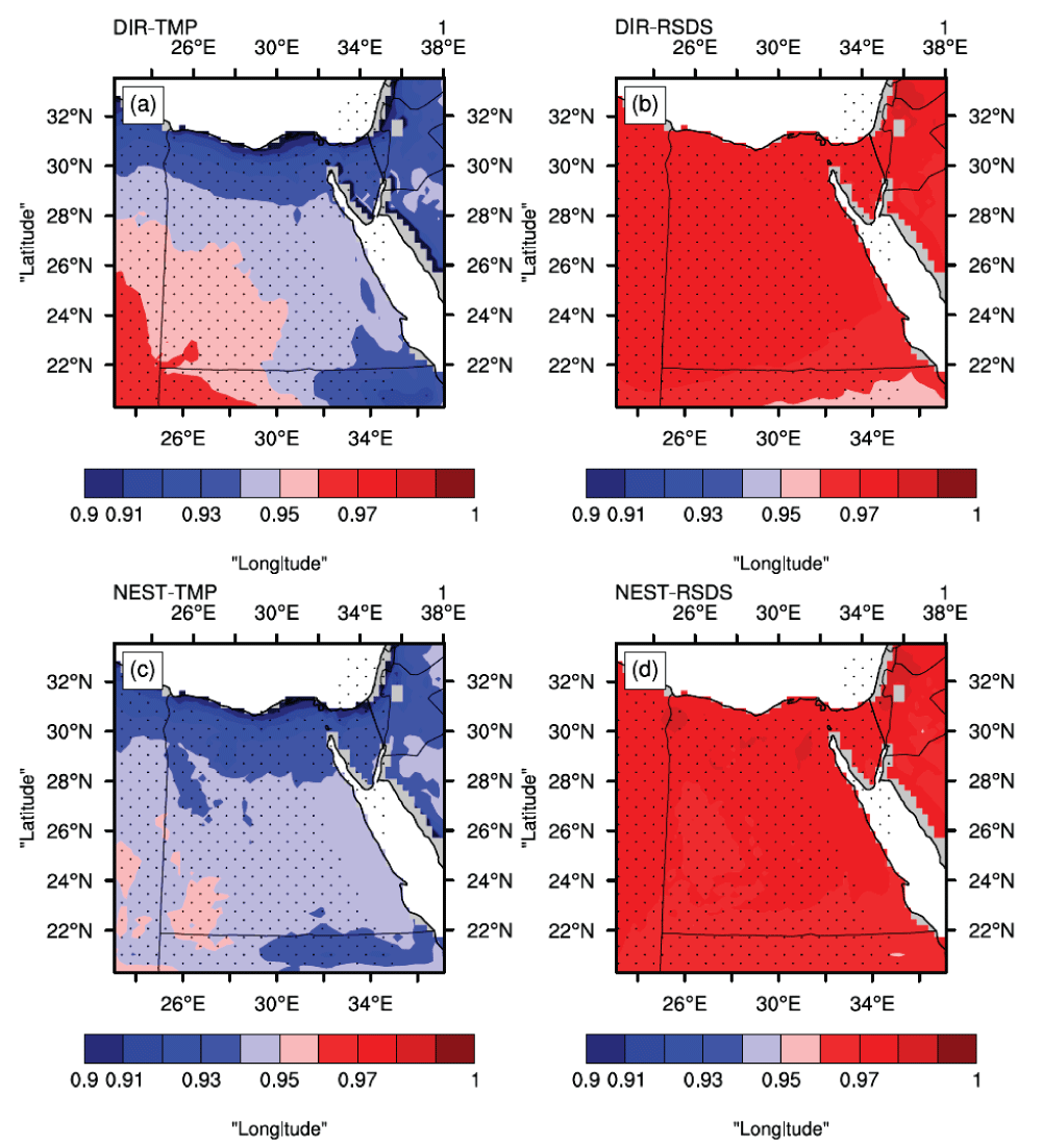
In section (3.1), it was found that PET is iNSEnsitive to the option of the dynamical downscaling or the boundary layer scheme despite the noted changes to the TMP. This point can be attributed to the fact that RSDS is not affected by any of the two cases. Therefore, it was suggested that the RSDS is the main driver controlling the PET changes followed by the TMP. To confirm this point, a regional map of the Pearson correlation coefficient [59] was plotted between the PET, RSDS, and TMP for each case. Figure 4a shows the correlation between PET and TMP, while the correlation between PET and RSDS is indicated in Figure 4b concerning the DIR simulation. In Figure 4a, it can be observed that the correlation between PET and TMP exhibits a gradient that differs with the region being examined. For instance, in the region of 30 °N - 32 °N, the gradient of PET - TMP correlation ranges between 0.9 and 0.94. While in the region of 22 °N - 28 °N, the correlation ranges between 0.94 and 0.96. Regarding the PET – RSDS dependence, it can be seen that the correlation is between 0.96 and 0.98 (Figure 4c). For the NEST simulation, the PET–TMP dependence is quite different from the one observed in the DIR simulation because NEST is warmer than DIR in all seasons [31]. This point can be indicated by noting that the correlation in this case ranges between 0.9 and 0.95 (Figure 4c). As for the RSDS, the situation is not quite different from the DIR simulation because RSDS does not change between the two simulations. Therefore, it can be observed that the correlation ranges from 0.96 to 0.98, similar to the DIR simulation (Figure 4d).

Figure 4: Pearson correlation coefficient for each grid point for DIR (a for TMP), (b for RSDS); NEST (c for TMP), and (d for RSDS). Note that the range of 0.9 and 1 has been chosen after many trials to choose the appropriate range.

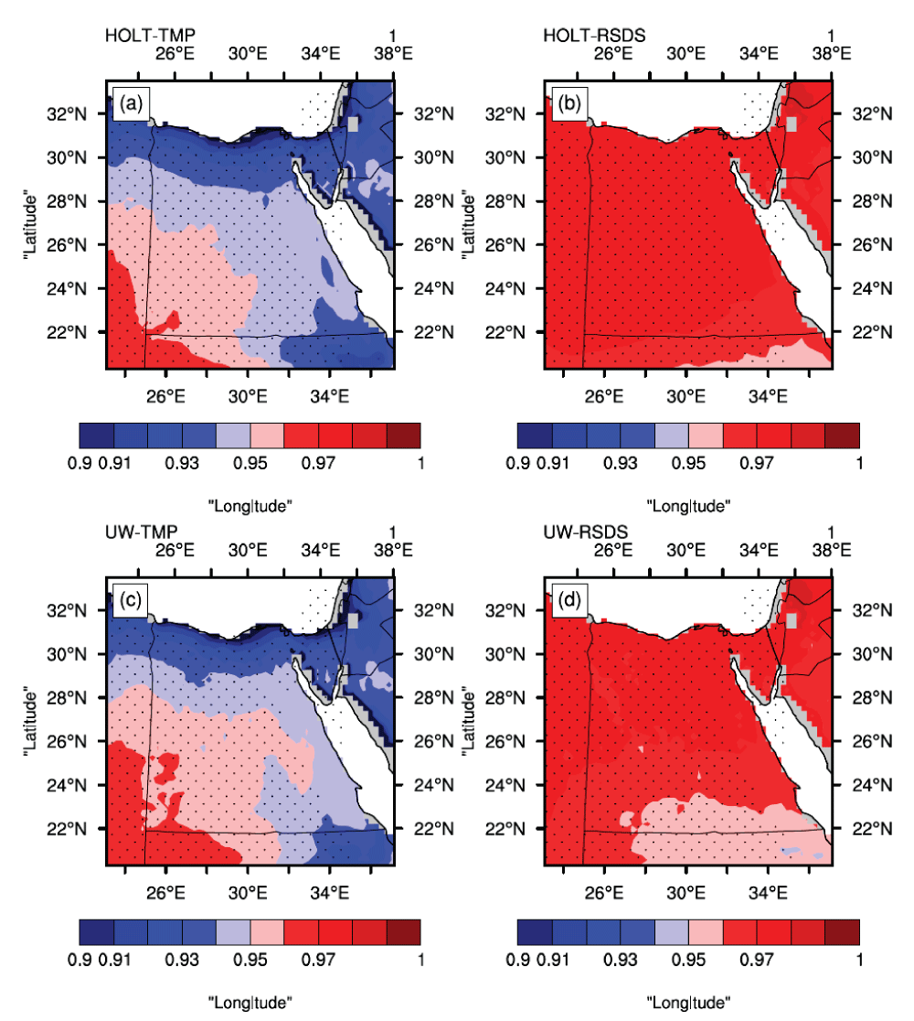
Concerning the case of the boundary layer parameterization, the PET–TMP correlation does not vary much between the boundary layer schemes (Figure 5 a, c) compared to the case of dynamical downscaling. For instance, the correlation (in the two simulations HOLT and UW) ranges between 0.9 and 0.96. This noted behavior can be attributed to two reasons: 1) the difference between DIR and NEST is larger than HOLT and UW and 2) regarding TMP changes between HOLT and UW, RSDS is the main driver of PET changes followed by TMP. Regarding RSDS, there is only a 1% difference between the correlations of the two simulations. For example, for the HOLT simulation (Figure 5c), the correlation is between 0.96 and 0.98. On the other hand, the correlation ranges between 0.95 and 0.98 (Figure 5d) for the UW simulation.

Figure 5: Pearson correlation coefficient for each grid point for HOLT (a for TMP), (b for RSDS); UW (c for TMP), and (d for RSDS). Note that the range of 0.9 and 1 has been chosen after many trials to choose the appropriate range.

Climatological annual cycle of PET

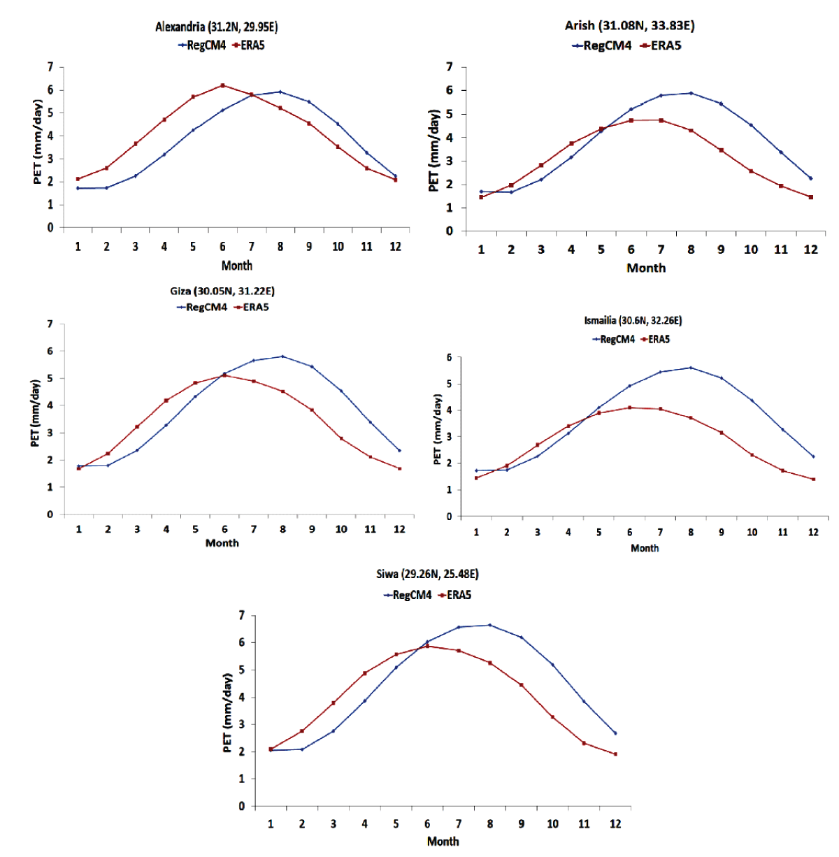
To evaluate the simulated PET (on a point scale), the combination of DIR–UW (referred to as RegCM4) has been considered based on the recommendation of [34]. The climatological annual cycle of the PET was evaluated concerning ERA5 (at locations of [18]) except for Port-Said and Marsa-Matruh as discussed in section (2.3). Preliminary analysis indicated that the simulated annual cycle can be categorized as phase (Figure 6) and non-phase shift (Figure 7).

Figure 6: Climatological annual cycle of the simulated PET concerning the ERA5 for the locations: Alexandria, Arish, Giza, Ismaila and Siwa.

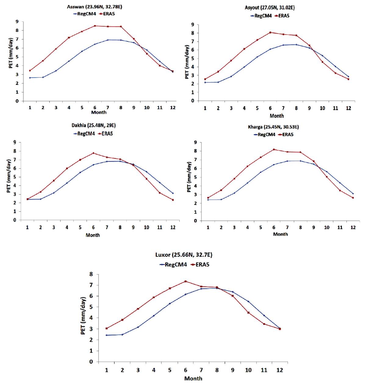
Figure 7: Climatological annual cycle of the simulated PET concerning the ERA5 for the locations: Asswan, Asyout, Dakhla, Kharga, and Luxor.

This means that in the phase shift, the simulated PET maximum value is either delayed or advanced concerning the ERA5. On the other hand, the non-phase-shift considers consistency in the PET maximum value between RegCM4 and ERA5. Each phase comprises five stations. For instance, Figure 6 shows the annual cycle of the simulated PET (in comparison with the ERA5) for the locations: Alexandria, Arish, Giza, Ismaila, and Siwa. On the other hand, Figure 7 considers the comparison between the simulated PET and ERA5 for the locations: Asswan, Asyout, Dakhla, Kharga, and Luxor. Figure 6 shows that the RegCM4 underestimates the PET (from January to June), while it overestimates the PET during the rest of the months in Alexandria. Additionally, RegCM4’s peak lies in August and ERA5’s peak occurs in June. The three locations (Arish, Giza, Ismaila, and Siwa) share a common feature regarding RegCM4’s behavior concerning the ERA5. For instance, in the aforementioned locations, the RegCM4 is close to the ERA5 from January to May, while the RegCM4 overestimates the PET during the rest of the months. Like Alexandria, RegCM4’s peak occurs in August, while the ERA5’s peak is in June. In Giza, RegCM4’s peak occurs in July and August, while ERA5’s peak occurs in June and July.

From Figure 6, it can be noted that the RegCM4 model has a limited ability to reproduce the climatological annual cycle of the simulated PET with the ERA5 for the coastal locations (Alexandria, Arish, Ismaila, and Siwa) and near-coast locations (Giza). In Figure 7, the situation is different because the RegCM4 can reproduce the simulated annual cycle of the PET compared to the ERA5. For instance, both the RegCM4 and ERA5 show the PET’s peak during June, July, and August. Additionally, the RegCM4 underestimates the PET from January to August, while the RegCM4 is close to the ERA5 during the rest of the months. The noted behavior in Figures 6 and 7 can be attributed to calibrating the radiation coefficient of the HS equation [36]. Although the calibrated HS equation succeeded in reducing the PET bias (compared to the original version), in some locations the values of the calibrated PET value are less than the one noted in the ERA5 (particularly in Figure 6). Additionally, Anwar and Lazic [36] reported that the added value of the calibrated HS equation depends on the location of the study.

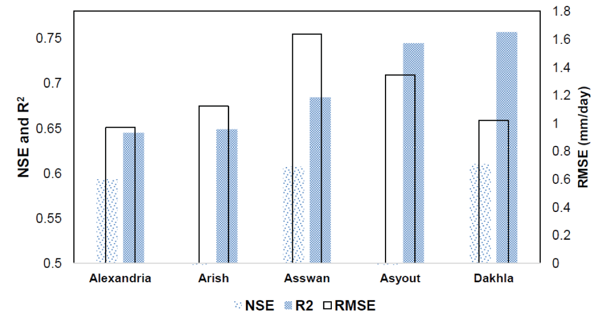
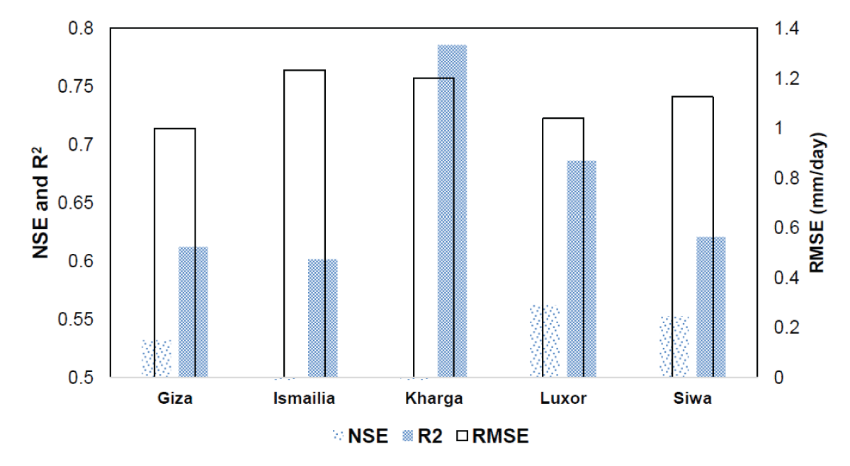
Figure S1 shows the statistical metrics (reported in section 2.2) for the simulated PET concerning the ERA5. From Figure S1, it can be noted that R² shows a gradual increase, Alexandria is the lowest one (R² ranges from 0.5 to 0.6), while Dakhla shows the highest record (R² ranges from 0.5 to 0.75). Concerning RMSE, it can be noted that Asswan has the highest form (RMSE = 1.6 mm day^-1), followed by Asyout and then Arish. For Alexandria and Dakhla, both locations show RMSE of ~1 mm day^-1. Additionally, NSE shows distinctive values among the locations above. For instance, the NSE for Alexandria, Asswan, and Dakhla ranges between 0.5 and 0.6. On the other hand, the NSE (of Arish and Asyout) equals ~0.5. In Figure S2, it can be observed that RMSE (among the indicated locations) ranges between 1 and 1.2 mm day^-1. Regarding R², Kharga has the highest records (R² ranges from 0.5 to 0.79), followed by Luxor and Siwa. On the other hand, Giza and Ismailia have the lowest records of R² (0.5 to 0.6). Compared to Figure S1, the NSE shows low values (~0.2 for Giza, Luxor, and Siwa; around zero for Ismailia and Kharga). Figures S1 and S2 show, it can be seen that NSE is relatively low (0.2 to 0.6 depending on the location). Also, R² is quite low for the majority of locations (0.5 to 0.6). Finally, RMSE is quite high (1 to 1.6 mm day^-1). Therefore, the LS technique can be could appropriate solution for reducing the RMSE and increasing the NSE and R². In section 3.4, the added value of the LS (either in the evaluation or the validation period) will be investigated.

Figure S1: Shows various statistical metrics: NSE, R², and RMSE for the locations: Alexandria, Arish, Asswan, Asyout, and Dakhla.

Figure S2: Shows various statistical metrics: NSE, R², and RMSE for the locations: Giza, Ismailia, Kharga, Luxor, and Siwa.

Added value of the LS method

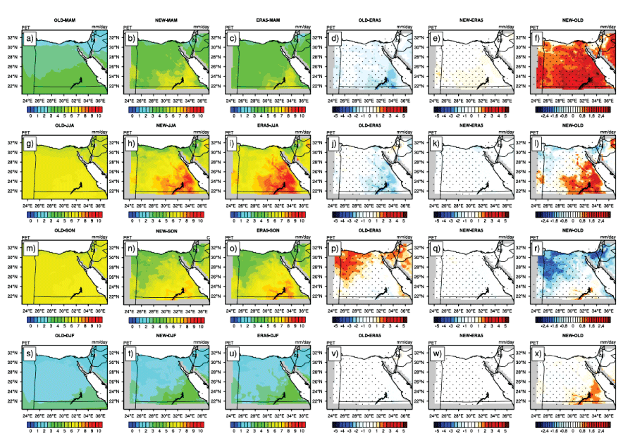
As reported in sections (3.1 and 3.3), the simulated PET is subjected to a notable bias regardless of the simulation configuration (DIR/NEST or HOLT/UW). Therefore, the LS method has been applied to possibly reduce the RegCM4 bias. Following the LS method (section 2.2), the climatological RegCM4 bias has been applied for each season to the output of the DIR-UW configuration (as recommended by [34]) considering 1998 – 2008 as the evaluation period. Figure 8 shows the seasonal climatology of the simulated PET before applying the LS (OLD) and after considering the LS (NEW) concerning the ERA5 as well as the difference between NEW and OLD in each season. From Figure 7, it can be noted that the LS not only proves its efficiency in reducing the PET bias but also improves the capability of the RegCM4 to better capture the PET spatial pattern in all seasons (Figure 8 a-c; g–i; m–o; s–u). Concerning the PET bias, the efficiency of the LS varies with the season of study.

In the MAM season, the PET bias ranges from -0.5 mm to -2.5 mm day^-1 when the LS is not applied (Figure 8d). On the other hand, the bias becomes around +0.5 mm day^-1 after considering the LS (Figure 8e). Qualitatively, the corrected PET is higher than the uncorrected one by ~2.5 mm day^-1 (Figure 8f). In the JJA, the NEW shows its potential skills in a better ability to capture the spatial pattern of the simulated PET (Figure 8h) than the OLD (Figure 8i), particularly around Nasser Lake. The RegCM4 bias (before and after considering the LS) is similar to the one observed in the MAM (Figure 8 j, k), particularly in the region of 22 – 28°N (Figure 8l). In the SON season, the situation is quite different from the one noted in the MAM and JJA because the OLD shows a 1 – 2.5 mm day^-1 bias mainly in the northwest region (Figure 8p). On the other hand, the NEW shows a bias of ±0.5 mm day^-1 (Figure 8q). That is why the NEW is lower than OLD by ~3 mm day^-1 (Figure 8r). Finally, in the DJF, there is no notable difference between OLD and NEW (Figure 8 v, w) except for Lake-Nasser where the LS method showed its efficiency in the reduction of the negative bias (Figure 8x).

Figure 8: Potential evapotranspiration over the period 1998–2008 (PET; in mm day-1) for MAM season in the first row (a - f); JJA in the second (g - l); SON in the third (m - r); and DJF in the fourth (s - x). For each row, OLD is on the left, followed by NEW; ERA5 is the third from left, OLD minus ERA5, NEW minus ERA5, and the difference between NEW and OLD. Significant difference/bias is indicated in black dots using a student t-test with alpha equal to 5%. Please note that OLD refers to the simulated PET before applying the Delta method; while NEW is the simulated PET after applying the Delta method.

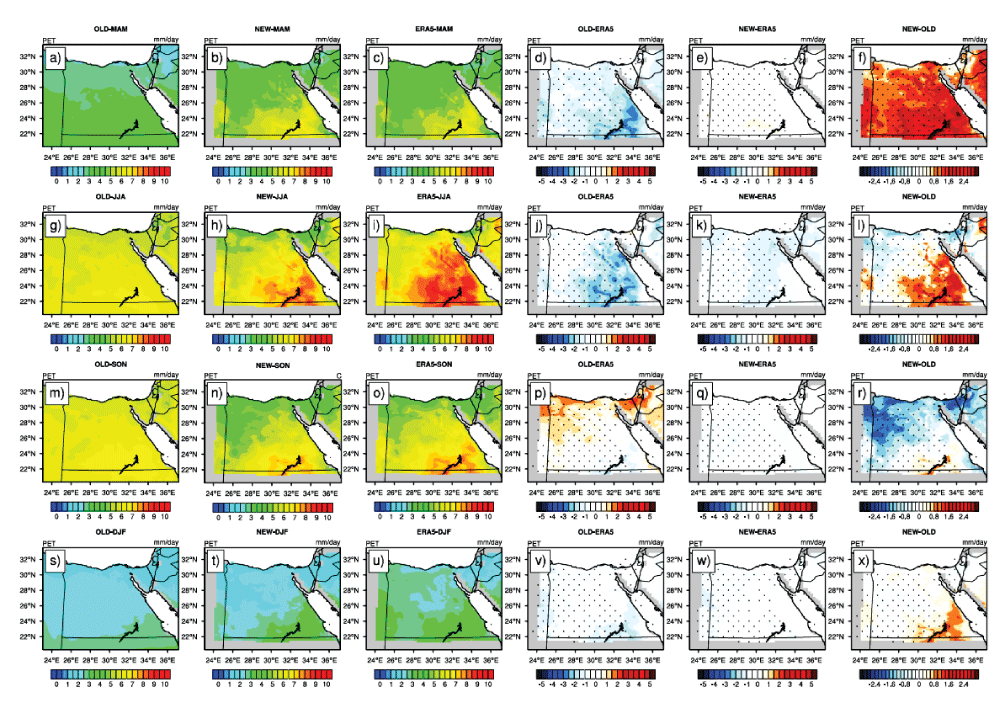
The added value of the LS was further tested in the validation period (Figure 9). As reported in section (2.2), the climatological bias (of each season) of 1998 – 2008 has been added to the RegCM4 raw data of 2009 – 2017. Like Figure 8, the NEW shows its potential skills for reproducing the PET spatial pattern than OLD in all seasons (Figure 9 a-c; g – i; m – o; s – u). However, the PET biases differ from those noted in Figure 8. For instance, the NEW shows a near zero bias except for Lake Nasser where the bias ranges from +0.5 to +1 mm day^-1 in the MAM season (Figure 9e). Also, NEW is higher than OLD by 0.8 – 3 mm day^-1 (Figure 9f). In the JJA, the OLD shows a bias of -1 to -3 mm day^-1 (Figure 9j), while the NEW has a bias of -0.5 to -1 mm day^-1 (Figure 9k). The difference between OLD and NEW (Figure 9l) is quite similar to the one observed in Figure 8l. Additionally, the RegCM4 behavior (in the SON and DJF; Figure 9 p, q, v, w) is similar to the one noted in Figure 8. The same concept applies to the difference between NEW and OLD (Figure 9 r, x).

Figure 9: Potential evapotranspiration over the period 2009–2017 (PET; in mm day-1) for MAM season in the first row (a - f); JJA in the second (g - l); SON in the third (m - r); and DJF in the fourth (s - x). For each row, OLD is on the left, followed by NEW; ERA5 is the third from left, OLD minus ERA5, NEW minus ERA5, and the difference between NEW and OLD. Significant difference/bias is indicated in black dots using a student t-test with alpha equal to 5%. Please note that OLD refers to the simulated PET before applying the Delta method; while NEW is the simulated PET after applying the Delta method.

Discussion

One must accurately estimate potential evapotranspiration (PET) to gauge crop water needs and carefully monitor agricultural and meteorological droughts. Allen, et al. [7] supported the application of the PM equation for PET estimates in the pursuit of such accuracy. In addition, Awal, et al. [60] pointed out that the PM equation is difficult since it requires a lot of atmospheric variables that might not be easily accessible in terms of space or time. This is due to the PM equation’s demanding nature regarding data collecting. Due to this situation, researchers have been scrambling to find an alternate method for PET estimates that depends more on an empirical approach and less on meteorological inputs [19,36,49,60]. But when compared to PM measurements, the uncorrected version of this empirical equation could only sometimes produce accurate PET estimates and might even produce over- or underestimations. The search for localized calibration, customized to the particular study region, thus becomes a critical answer. Such calibration makes it possible to approximate the accuracy of PET estimates rationally.

Focusing mainly on the HS equation, which replaces the PM model, its calibration has shown notable effectiveness across numerous geographical locations. There are notable examples in West Texas [60], Eastern India [21], Nigeria [61], and the Sudan and South Sudan [19]. This demonstrates how flexible and useful the equation is across various global locations. Furthermore, it’s critical to recognize that assuring computed PET accuracy depends not only on the calibration of the empirical equation but also on the setup of the regional climate model (such as RegCM4) used for this. For instance, Xu, et al. [30] highlighted that direct downscaling with finer resolution can greatly improve RegCM4’s accuracy. When it comes to replicating mean air temperature and total surface precipitation, this method performs better than the coarser resolution and even outperforms the two-way nesting strategy.

In Egypt, a comparison has been conducted between direct downscaling and one-way nesting investigating its influence on the daily mean air temperature [31]. In this study, Anwar [31] found that direct downscaling (DIR) outperforms one-way nesting (NEST); such performance was indicated by a low bias of direct downscaling compared to one-way nesting (in which the RegCM4 bias has been amplified). Additionally, the accuracy of the RegCM4 has been examined by various schemes of the boundary layer [34]. In this study, the authors reported that the UW scheme is better than the HOLT in simulating the daily mean air temperature concerning the ERA5. However, the influence of dynamical downscaling options or the role of the boundary layer schemes has not been examined for the PET of Egypt until the present day.

The present study closely examined how Egypt’s simulated Potential Evapotranspiration (PET) responded to a range of dynamical downscaling options and boundary layer techniques using the RegCM4 regional climate model. We performed a thorough analysis of RegCM4 outputs throughout many seasons, examining them at both regional and annual scales, with a focus on the ERA5-land-based reanalysis product (hPET). Additionally, the efficiency of the LS bias-correction method underwent thorough evaluation and validation. The results showed that neither the dynamical downscaling options nor the boundary layer techniques affected the simulated PET. This shows that RSDS, followed by TMP, is what predominantly affects the PET changes. To improve the simulated PET in the current climate or various future scenarios, the climatological bias of each season might be added to the RegCM4 raw output data about the LS potential skills.

Conclusion and future work

In conclusion, the RegCM4 can be used to develop a PET map of Egypt using the DIR-UW configuration and LS bias correction technique (for each season). This finding not only aids policymakers in assessing the daily water requirements of crops, which is crucial for daily forecasts, especially in regions with limited data but also holds the potential for projecting future water needs under varying warming scenarios. Such insights provide a vital resource for strategic decision-making in agricultural and water resource management, offering a bridge between scientific advancement and actionable policies.

It is important to highlight an important point; the climatological bias factor (section 3.4) can be used in periods to reasonably estimate the PET (particularly in data-scarce regions). In comparison with previous literature reviews, the present study offers a novel way to accurately estimate the PET through the RegCM4 regional climate model and LS method. However, it should be noted that the impact of aerosols on the RSDS budget and, coNSEquently, the simulated PET, was not taken into account in this study. Therefore, the following points will be covered: 1 – include the aerosol effects, 2 – study the influence of lateral boundary conditions (provided by the Fifth/Sixth Coupled Model Intercomparison Project (CMIP5/CMIP6), and 3 - use a convection-permitting resolution and a new dynamical core (i.e., RegCM5).

Supplementary materials

The present study has two supplementary figures: Figure S1 shows various statistical metrics: NSE, R², and RMSE for the locations: Alexandria, Arish, Asswan, Asyout, and Dakhla; Figure S2 shows various statistical metrics: NSE, R², and RMSE for the locations: Giza, Ismailia, Kharga, Luxor and Siwa.

Author contributions

Conceptualization, S.A.A.; methodology, S.A.A.; software, S.A.A.; validation, S.A.A.; formal analysis, S.A.A. and A.S.; investigation, S.A.A. and A.S.; resources, S.A.A.; data curation, S.A.A.; writing—original draft preparation, S.A.A. and A.S.; writing—review and editing, S.A.A. and A.S.; visualization, S.A.A. and A.S.; supervision, S.A.A. and A.S.; project administration, S.A.A. All authors have read and agreed to the published version of the manuscript.

Acknowledgment

The Egyptian Meteorological Authority (EMA) is acknowledged for providing the computational power to conduct the model simulations. Hourly potential evapotranspiration (hPET) was retrieved from the web link https://data.bris.ac.uk/data/dataset/qb8ujazzda0s2aykkv0oq0ctp. However, the monthly mean can be acquired from the authors upon request (accessed on 18 October 2022).

References

1. Climate Change 2007: Synthesis Report. IPCC 2007. Technical report, IPCC.

2. Climate change 2014: impacts, adaptation, and vulnerability. Cambridge University Press, New York; 2014.

3. Wilco T, Walter WI, Peter D. Climate change projections of precipitation and reference evapotranspiration for the Middle East and Northern Africa until 2050. Int J Climatol. 2013;33:3055-3072. https://doi.org/10.1002/joc.3650.

4. Gurara MA, Jilo NB, Tolche AD. Impact of climate change on potential evapotranspiration and crop water requirement in Upper Wabe Bridge watershed, Wabe Shebele River Basin, Ethiopia. J Afr Earth Sci. 2021;180:104223.

5. Allen RG, Smith M, Pereira LS, Perrier A. An update for the calculation of reference evapotranspiration. ICID Bulletin. 1994;43:35-92.

6. Hamed MM, Iqbal Z, Nashwan MS, Kineber AF, Shahid S. Diminishing evapotranspiration paradox and its cause in the Middle East and North Africa. Atmos Res. 2023;289:106760. https://doi.org/10.1016/j.atmosres.2023.106760.

7. Allen GR, Pereira LS, Raes D, Smith M. Crop Evapotranspiration: Guidelines for Computing Crop Water Requirements; Report 56; Food and Agricultural Organization of the United Nations (FAO): Rome, Italy; 1998;300.

8. Sperna Weiland FC, Tisseuil C, Dürr HH, Vrac M, van Beek LPH. Selecting the optimal method to calculate daily global reference potential evaporation from CFSR reanalysis data for application in a hydrological model study. Hydrol Earth Syst Sci. 2012;16:983-1000. www.hydrol-earth-syst-sci.net/16/983/2012.

9. Murat C, Hatice C, Tefaruk H, Kisi O. Modifying Hargreaves-Samani equation with meteorological variables for estimation of reference evapotranspiration in Turkey. Hydrol Res. 2017;48(2):480-497. https://doi.org/10.2166/nh.2016.217.

10. Hargreaves GL, Allen RG. History and evaluation of Hargreaves evapotranspiration equation. J Irrigat Drain Eng. 2003;129:53-63.

11. ElNesr MN, Alazba AA, Amin MT. Modified Hargreaves’ Method as an Alternative to the Penman-monteith Method in the Kingdom of Saudi Arabia. Aust J Basic Appl Sci. 2011;5(6):1058-1069.

12. Raziei T, Pereirab LS. Estimation of ETo with Hargreaves–Samani and FAO-PM temperature methods for a wide range of climates in Iran. Agric Water Manag. 2013;121:1-18.

13. Kumari N, Srivastava A. An Approach for Estimation of Evapotranspiration by Standardizing Parsimonious Method. Agric Res. 2020;9:301-309.

14. Incoom ABM, Adjei KA, Odai SN, Akpoti K, Siabi EK. Impacts of climate change on crop and irrigation water requirement in the Savannah regions of Ghana. J Water Clim Chang. 2022;13(9):3338-3356. https://doi.org/10.2166/wcc.2022.129.

15. Er-Raki S, Chehbouni A, Khabba S, Simonneaux V, Jarlan L, Ouldbba A, et al. Assessment of reference evapotranspiration methods in semi-arid regions: can weather forecast data be used as alternate of ground meteorological parameters? J Arid Environ. 2010;74(12):1587-1596.

16. Li Z, Yang Y, Kan G, Hong Y. Study on the Applicability of the Hargreaves Potential Evapotranspiration Estimation Method in CREST Distributed Hydrological Model (Version 3.0) Applications. Water. 2018;10:1882. https://doi.org/10.3390/w10121882.

17. Terink W, Immerzeel WW, Droogers P. Climate change projections of precipitation and reference evapotranspiration for the Middle East and Northern Africa until 2050. Int J Climatol. 2013;33:3055-3072. https://doi.org/10.1002/joc.3650.

18. Anwar SA, Salah Z, Khaled W, Zakey AS. Projecting the Potential Evapotranspiration in Egypt Using a High-Resolution Regional Climate Model (RegCM4). Environ Sci Proc. 2022;19:43. https://doi.org/10.3390/ecas2022-12841.

19. Elagib NA, Musa AA. Correcting Hargreaves-Samani formula using geographical coordinates and rainfall over different timescales. Hydrol Process. 2022;37. https://doi.org/10.1002/hyp.14790.

20. Srivastava A, Sahoo B, Raghuwanshi NS, Singh R. Evaluation of variable-infiltration capacity model and MODIS-terra satellite-derived grid-scale evapotranspiration estimates in a River Basin with Tropical Monsoon-Type climatology. J Irrig Drain Eng. 2017;143(8):04017028.

21. Srivastava A, Sahoo B, Raghuwanshi NS, Chatterjee C. Modelling the dynamics of evapotranspiration using Variable Infiltration Capacity model and regionally calibrated Hargreaves approach. Irrig Sci. 2018;36:289-300. https://doi.org/10.1007/s00271-018-0583-y.

22. Spinoni J, Barbosa P, Bucchignani E. Global exposure of population and land-use to meteorological droughts under different warming levels and SSPs: A CORDEX-based study. Int J Climatol. 2021;41(15):6825-6853. https://doi.org/10.1002/joc.7302.

23. Almorox J, Grieser J. Calibration of the Hargreaves–Samani method for the calculation of reference evapotranspiration in different Köppen climate classes. Hydrol Res. 2016;47(2):521-531. https://doi.org/10.2166/nh.2015.091.

24. Giménez PO, García-Galiano SG. Assessing Regional Climate Models (RCMs) Ensemble-Driven Reference Evapotranspiration over Spain. Water. 2018;10(9):1181. https://doi.org/10.3390/w10091181.

25. Gurara MA, Jilo NB, Tolche AD. Impact of climate change on potential evapotranspiration and crop water requirement in Upper Wabe Bridge watershed, Wabe Shebele River Basin, Ethiopia. J Afr Earth Sci. 2021;180:104223.

26. Raziei T, Pereirab LS. Estimation of ETo with Hargreaves–Samani and FAO-PM temperature methods for a wide range of climates in Iran. Agric Water Manag. 2013;121:1-18.

27. Remrová M, Císlerová M. Analysis of Climate Change Effects on Evapotranspiration in the Watershed Uhlířská in the Jizera Mountains. Soil Water Res. 2010;5(1):28-38.

28. Vahmani P, Jones AD, Li D. Will anthropogenic warming increase evapotranspiration? Examining irrigation water demand implications of climate change in California. Earth's Future. 2022;10. https://doi.org/10.1029/2021EF002221.

29. Chen L, Huang G, Wang X. Projected changes in temperature, precipitation, and their extremes over China through the RegCM. Clim Dyn. 2019;53(9):5859-5880. https://doi.org/10.1007/s00382-019-04899-7.

30. Xu X, Huang A, Huang Q. Impacts of the horizontal resolution of the lateral boundary conditions and downscaling method on the performance of RegCM4.6 in simulating the surface climate over central-eastern China. Earth Space Sci. 2022;9. https://doi.org/10.1029/2022EA002433..

31. Anwar SA. Influence of Direct-Downscaling and One-Way Nesting on Daily Mean Air Temperature of Egypt Using the RegCM4. J Basic Res Eng Sci. 2023 Mar 09;4(3):338-347. doi:10.37871/jbres1681. Available at: https://www.jelsciences.com/articles/jbres1681.pdf.

32. Ali MFA, Salah Z, Asklany SA, Hassan M, Harhash M, Wahab MMA. A Comparison of Three Boundary Layer Schemes for Numerical Weather Prediction. Appl Math Inf Sci. 2020;14(6):1093-1101. http://dx.doi.org/10.18576/amis/140616.

33. Holtslag AAM, Boville BA. Local versus nonlocal boundary layer diffusion in a global model. J Clim. 1993;6:1825-1842.

34. Anwar SA, Mostafa SM. On the Sensitivity of the Daily Mean Air Temperature of Egypt to Boundary Layer Schemes Using a High-Resolution Regional Climate Model (RegCM4). J Basic Res Eng Sci. 2023 Mar 22;4(3):474-484. doi:10.37871/jbres1700. Available at: https://www.jelsciences.com/articles/jbres1700.pdf.

35. Grenier H, Bretherton CS. A moist PBL parameterization for large scale models and its application to subtropical cloud-topped marine boundary layers. Mon Weather Rev. 2001;129:357-377.

36. Anwar SA, Lazić I. Estimating the Potential Evapotranspiration of Egypt Using a Regional Climate Model and a High-Resolution Reanalysis Dataset. Environ Sci Proc. 2023;25:29. https://doi.org/10.3390/ECWS-7-14253.

37. Lafon T, Dadson S, Buys G, Prudhomme C. Bias correction of daily precipitation simulated by a regional climate model: A comparison of methods. Int J Climatol. 2013;33:1367-1381.

38. El Kenawy A, Lopez-Moreno JI, Vicente-Serrano SM, Morsi F. Climatological modeling of monthly air temperature and precipitation in Egypt through GIS techniques. Clim Res. 2010;42:161-176.

39. Nashwan MS, Shahid S. Symmetrical uncertainty and random forest for the evaluation of gridded precipitation and temperature data. Atmos Res. 2019;230:104632.

40. Peel MC, Finlayson BL, McMahon TA. Updated World Map of the Köppen-Geiger Climate Classification. Hydrol Earth Syst Sci. 2007;11:1633-1644.

41. Dickinson RE, Errico RM, Giorgi F, Bates GT. A regional climate model for the western United States. Clim Change. 1989;15:383-422.

42. Giorgi F, Bates GT. The climatological skill of a regional model over complex terrain. Mon Wea Rev. 1989;117:2325-2347.

43. Giorgi F. Thirty years of regional climate modeling. Where are we and where are we going? J Geophys Res. 2019;124:5696-5723.

44. Giorgi F, Marinucci MR, Bates GT. Development of a second generation regional climate model (RegCM2). Part I: Boundary layer and radiative transfer processes. Mon Wea Rev. 1993;121:2794-2813.

45. Giorgi F, Marinucci MR, Bates GT, DeCanio G. Development of a second generation regional climate model (RegCM2). Part II: Convective processes and assimilation of lateral boundary conditions. Mon Wea Rev. 1993;121:2814-2832.

46. Pal JS, Giorgi F, Bi X, Elguindi N, Solmon F, Gao X, et al. The ICTP RegCM3 and RegCNET: Regional climate modeling for the developing World. Bull Amer Meteor Soc. 2007;88:1395-1409.

47. Giorgi F, Coppola E, Solmon F, Mariotti L, Sylla MB, Bi X, et al. RegCM4: model description and preliminary tests over multiple CORDEX domains. Clim Res. 2012;52:7-29.

48. Giorgi F, Coppola E, Giuliani G, Ciarlo` JM, Pichelli E, Nogherotto R, et al. The Fifth Generation Regional Climate Modeling System, RegCM5: Description and Illustrative Examples at Parameterized Convection and Convection-Permitting Resolutions. J Geophys Res Atmos. 2023. Available from: https://doi.org/10.1029/2022JD038199.

49. Anwar SA, Malcheva K, Srivastava A. Estimating the potential evapotranspiration of Bulgaria using a high‑resolution regional climate model. Theor Appl Climatol. 2023. Available from: https://doi.org/10.1007/s00704-023-04438-9.

50. Anwar SA, Mamadou O, Diallo I, Sylla MB. On the influence of vegetation cover changes and vegetation-runoff systems on the simulated summer potential evapotranspiration of tropical Africa using RegCM4. Earth Syst Environ. 2021;5:883-897. https://doi.org/10.1007/s41748-021-00252-3.

51. Anwar SA, Diallo I. A RCM investigation of the influence of vegetation status and runoff scheme on the summer Gross Primary Production of Tropical Africa. Theor Appl Climatol. 2021;145:1407-1420. https://doi.org/10.1007/s00704-021-03667-0.

52. Anwar SA, Diallo I. Modelling the Tropical African Climate using a state-of-the-art coupled regional climate-vegetation model. Clim Dyn. 2022;58:97-113.

53. Dee DP, Uppala SM, Simmons AJ, Berrisford P, Poli P, Kobayashi S, et al. The ERA-Interim reanalysis: configuration and performance of the data assimilation system. Q J R Meteorol Soc. 2011;137:553-597. https://doi.org/10.1002/qj.828.

54. Singer M, Asfaw D, Rosolem R, Cuthbert MO, Miralles DG, MacLeod D, et al. Michaelides K. Hourly potential evapotranspiration (hPET) at 0.1degs grid resolution for the global land surface from 1981-present. Sci Data. 2021;8:224. https://doi.org/10.1038/s41597-021-01003-9.

55. Nashwan MS, Shahid S, Chung ES. High-Resolution Climate Projections for a Densely Populated Mediterranean Region. Sustainability. 2020;12(9):3684. https://doi.org/10.3390/su12093684.

56. Mostafa SM, Anwar SA, Zakey AS, Wahab MMA. Bias-correcting the maximum and minimum air temperatures of Egypt using a high-resolution Regional Climate Model (RegCM4). Eng Proc. 2023;31:73. https://doi.org/10.3390/ASEC2022-13852.

57. Muñoz-Sabater J, Dutra E, Agustí-Panareda A, Albergel C, Arduini G, Balsamo G, et al. ERA5-Land: a state-of-the-art global reanalysis dataset for land applications. Earth Syst Sci Data. 2021;13:4349-4383. https://doi.org/10.5194/essd-13-4349-2021.

58. Harris I, Osborn TJ, Jones P, Lister D. Version 4 of the CRU TS monthly high-resolution gridded multivariate climate dataset. Sci Data. 2020 Apr 3;7(1):109. doi: 10.1038/s41597-020-0453-3. PMID: 32246091; PMCID: PMC7125108.

59. Kirch W. Pearson’s Correlation Coefficient. In: Kirch W, ed. Encyclopedia of Public Health. Springer; 2008. https://doi.org/10.1007/978-1-4020-5614-7_2569.

60. Awal R, Rahman A, Fares A, Habibi H. Calibration and Evaluation of Empirical Methods to Estimate Reference Crop Evapotranspiration in West Texas. Water. 2022;14:3032. https://doi.org/10.3390/w14193032.

61. Ogunrinde AT, Emmanuel I, Enaboifo MA, Ajayi TA, Pham QB. Spatio-temporal calibration of Hargreaves-Samani model in the Northern Region of Nigeria. Theor Appl Climatol. 2022;147:1213-1228. https://doi.org/10.1007/s00704-021-03897-2.

記事について

この記事を引用する

Anwar SA, Srivastava A. The Influence of Dynamical Downscaling and Boundary Layer Selection on Egypt’s Potential Evapotranspiration using a Calibrated Version of the Hargreaves-samani Equation: RegCM4 Approach. IgMin Res. July 24, 2024; 2(7): 646-661. IgMin ID: igmin229; DOI: 10.61927/igmin229; Available at: igmin.link/p229

• DOI10.61927/igmin229

11 Jul, 2024

受け取った

23 Jul, 2024

受け入れられた

24 Jul, 2024

発行された

この記事を共有する

次のリンクを共有した人は、このコンテンツを読むことができます:

共有リンクを取得する

トピックス

Environmental Sciences