Deep Learning-based Multi-class Three-dimensional (3-D) Object Classification using Phase-only Digital Holographic Information

Abstract

In this paper, we present a deep CNN-based approach for multi-class classification of three-dimensional (3-D) objects using phase-only digital holographic information. The 3-D objects considered for the multi-class (four-class) classification task are ‘triangle-square’, ‘circle-square’, ‘square-triangle’, and ‘triangle-circle’. The 3-D object ‘triangle-square’ is considered for Class-1 and the remaining 3-D objects ‘circle-square’, ‘square-circle’, and ‘triangle-circle’ are considered for Class-2, Class-3, and Class-4. The digital holograms of 3-D objects were created using the two-step Phase-Shifting Digital Holography (PSDH) technique and were computationally post-processed to obtain phase-only digital holographic data. Subsequently, a deep CNN was trained on a phase-only image dataset consisting of 2880 images to produce the results. The loss and accuracy curves are presented to validate the performance of the model. Additionally, the results are validated using metrics such as the confusion matrix, classification report, Receiver Operating Characteristic (ROC) curve, and precision-recall curve.

Introduction

Deep learning, a branch of artificial intelligence (AI), encompasses various deep neural networks, including Convolutional Neural Network (CNN), AlexNet, Visual Geometry Group (VGG) Networks, U-Net, Y-Net, and Convolutional Encoder-Decoder Network models. These networks have been utilized in various digital holographic applications, including focus prediction [1], depth prediction [2], image segmentation [3], hologram reconstruction [4], 3-D object binary classification [5], 3-D object binary regression [6,7], 3-D object multi-class classification and multi-output regression [8-10], and phase unwrapping [11]. Digital holography is an optical imaging technique that records 3-D information about an object using an electronic sensor such as a Charge-Coupled Device (CCD) or Complementary Metal Oxide Semiconductor (CMOS) sensor. The hologram recorded using a CCD sensor is numerically reconstructed to obtain a complex-valued image containing both intensity and phase information. This phase (depth) information can be utilized for AI-based supervised learning techniques such as classification and regression tasks. Classification is a supervised learning technique that defines the decision boundary between the input data and the target labels. The classification technique produces output as discrete labels. In this study, multi-class (four-class) classification of 3-D objects was performed using a deep CNN. A CNN is a deep neural network that consists of distinct layers for feature extraction and classification. The feature extraction component includes multiple convolutional and pooling layers. The convolutional layer performs a convolution operation between the input and the kernel to produce a feature map. This feature map is then processed through the pooling layer to reduce its dimensionality. The classification component comprises fully connected layers and an output layer to generate the final results. Zifei Li, et al. [12] introduced a deep CNN for binary classification of speckle patterns acquired from multi-mode fiber. Priscoli, et al. [13] explored both machine learning and deep learning techniques, including Principal Component Analysis (PCA), Multi-Layer Perceptron (MLP), and CNN, for binary classification of cancer cells in microfluidics. Additionally, Lam, et al. [14] proposed a deep CNN for hologram classification of occluded and deformable objects, addressing holograms contaminated with speckle noise. Cheng, et al. [15] introduced a deep CNN tailored for pattern classification of digital holographic data. Zhang, et al. [16] developed a deep CNN specifically for classifying marine plankton from digital holograms. Zhu, et al. [17] proposed an automated method for classifying microplastics in digital holographic data using deep learning and generative adversarial networks. The current study presents a multi-class (four-class) classification of 3-D objects, specifically ‘triangle-square’, ‘circle-square’, ‘square-triangle’, and ‘triangle-circle’, utilizing phase-only digital holographic information acquired from the Phase-Shifting Digital Holography (PSDH) technique through deep CNN. The primary distinction between this work and prior studies [12-17] lies in the utilization of deep CNN for multi-class (four-class) classification of 3-D objects based on phase-only digital holographic data acquired via phase-shifting digital holography. The results of the classification task are delineated in terms of loss and accuracy curves to validate the proof of concept. Furthermore, the work is validated with results including the confusion matrix, classification report, Receiver Operating Characteristic (ROC) curve, and precision-recall curve. Classifying phase images entails the classification of 3-D objects using deep CNN. The major contribution of this paper is this is the first work reported to perform a four-class classification of 3-D objects using phase-shifting digital holographic data.

Methodology

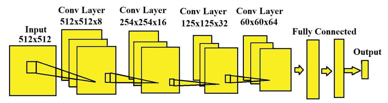
Figure 1 depicts a block diagram illustrating the CNN architecture employed for multi-class (four-class) classification of 3-D objects utilizing a phase-only image dataset. The CNN takes the input as the phase-only image of size 512 × 512 from the digital hologram. The CNN depicted in Figure 1 comprises four convolutional and four pooling layers in the feature extraction stage, followed by fully connected and output layers in the classification stage. In the convolutional layer, the input phase image undergoes convolution with a kernel to generate the feature map. The output of the convolutional layer is determined by

$Z_{pq}^{\left(k\right)}=P({\displaystyle {\sum }_{m=0}^t{\displaystyle \sum _{n=0}^t{H}_{mn}^{(k)}{X}_{pq}+B_{pq}}})$ (1)

In the above eqn. $Z_{pq}^{\left(k\right)}$ (1), represents the output feature map and X_pq represents the input phase image. $H_{mn}^{(k)}$ represents kernel coefficients, k represents the number of kernels, t represents the kernel size, P represents the activation function, and Bpq represents bias. The number of kernels in the convolutional layer is k = 8,16,32,64. The size of the kernel is t = 5 × 5. The activation function P represents the rectified linear unit (ReLU) activation function that is present in convolutional and fully connected layers. The output of the convolutional layer is then fed into the pooling layer, where the Max-Pooling2D technique is applied to further decrease the dimensionality of the feature map. The output of the pooling layer is determined by

Y_pq = X_pq (2)

In the above eqn. (2), Y_pq represents the output feature map and X_pq represents the input. The output of the final pooling layer is flattened and subsequently passed to the fully connected layer. The output of the fully connected layer is determined by

$Y_p=P({\displaystyle {\sum }_{p=1}^t{W}_{mn}{X}_p+B_p})$ (3)

In the above eqn. (3), Y_p represents the output of the fully connected layer, B_p represents the bias, P represents the ReLU activation function, W_mn represents weight values, X_p represents the one-dimensional (1-D) data obtained through the flattening layer, and t represents the number of neurons. The output of the final pooling layer is 28 × 28 × 64. The number of neurons selected in the fully connected layer is t = 64. The output of the fully connected layer is forwarded to the output layer. In the output layer, a subset of four neurons is selected from the sixty-four neurons, utilizing the softmax activation function to generate the final output. The equation for the softmax activation function is expressed as

$Q_K=\frac{\text{exp}(M_K)}{{{\displaystyle \sum }}_{n=1}^t\text{exp}(X_t)}$ (4)

In the above eqn. (4), Q_k represents the output, M_k represents the input, and t represents several neurons.

Dataset preparation

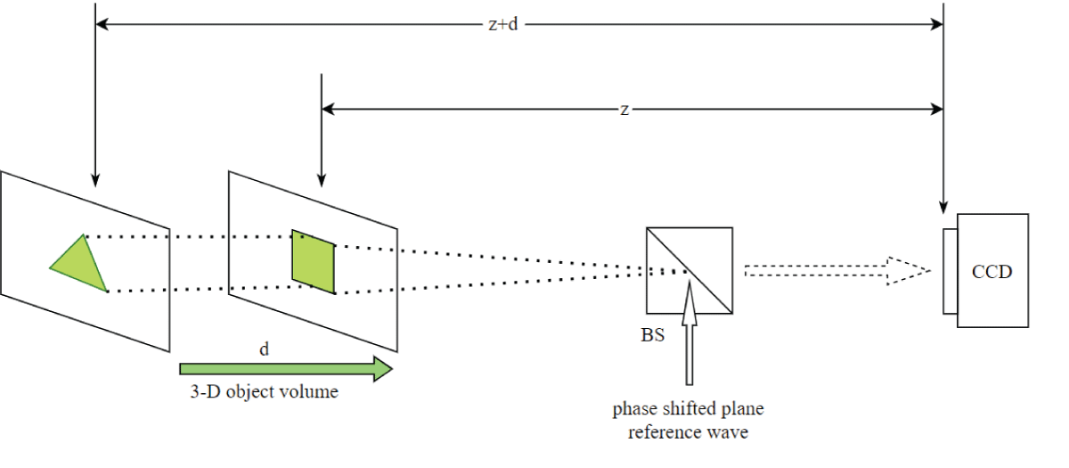
For the four-class classification task, the following four 3-D objects were included: ‘triangle-square’, ‘circle-square’, ‘square-triangle’, and ‘triangle-circle’. These objects were distributed among four distinct subclasses: Class-1, Class-2, Class-3, and Class-4. Specifically, the 3-D object ‘triangle-square’ was designated as belonging to Class-1. Following the classification scheme, the subsequent 3-D object, ‘circle-square’, was assigned to Class-2. Similarly, the 3-D object ‘square-triangle’ was allocated to Class 3. Finally, the last 3-D object, ‘triangle-circle’, was designated as belonging to Class-4. The 3-D object ‘circle-square’ was structured such that the circular feature resided prominently in the first plane, while the square feature was distinctly positioned in the subsequent plane. Each plane is separated by various distances d¹, and d² respectively. The remaining three 3-D objects were constructed similarly, with the distinction that different features were allocated to the first and second planes, respectively. Two phase-shifted holograms of 0⁰ and 90⁰ were formed at the camera plane and these holograms were post-processed to obtain a complex-valued image containing intensity and phase information using a two-step phase-shifting digital holography (PSDH) technique. The holograms and reconstructed intensity/phase images are of size 1024 × 1024. The intensity and phase images were reconstructed at both distances. In Figure 2a, a schematic representation of the 3-D object volume ‘triangle-square’, belonging to Class-1, is depicted, illustrating the distribution of information across both the first and second planes. Additionally, Figure 2a illustrates the geometry for digital hologram recording from two-step phase-shifted plane reference waves.

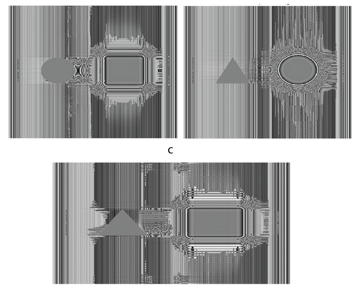
The digital holograms of four different 3-D objects namely ‘triangle-square’, ‘circle-square’, ‘square-triangle’, and ‘triangle-circle’ belonging to four-different sub-classes were further rotated in steps of 0.5° separately forming a dataset of 2880 holograms. Similarly, the reconstructed intensity/phase images obtained from the two-step Phase-Shifting Digital Holography (PSDH) technique were also rotated in steps of 0.5° to form a dataset of 2880 images separately for intensity and phase information. For the multi-class classification (four-class classification) of 3-D objects, only phase information was taken into account. The dataset, comprising 2880 phase images, was divided into training, validation, and test sets, containing 2160 (75%), 432 (15%), and 288 (10%) images, respectively. for the training of the deep CNN, the size of the phase image considered was 512 × 512 from 1024 × 1024. The deep CNN was trained for 50 epochs on the phase-only image dataset using an Adam optimizer with a learning rate of 0.0007, while categorical cross-entropy was employed as the loss function. The implementation of the deep CNN was carried out in a TensorFlow environment using Python programming. Figure 3 displays samples of three reconstructed phase images corresponding to 3-D objects, namely ‘triangle-square’, ‘circle-square’, and ‘triangle-circle’, which belong to Class-1, Class-2, and Class-4, respectively.

Results and discussions

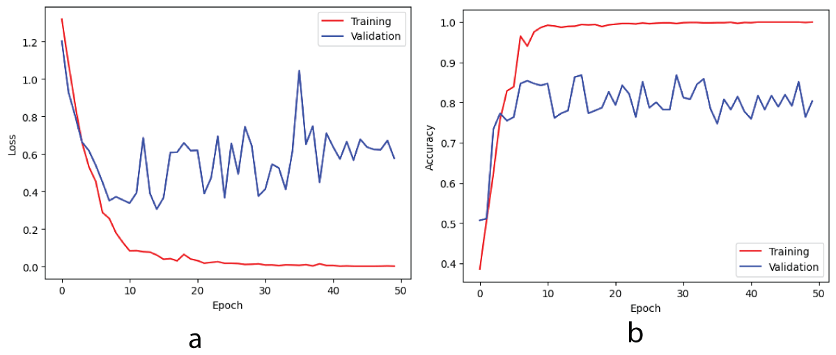
The deep CNN was trained on a batch of 54 images from the training set and a batch of 24 images from the validation set of the phase-only image dataset in a single epoch. Subsequently, each epoch was iteratively iterated over 40/18 steps on the training/validation sets to complete the training process. Figure 4 illustrates the loss/accuracy curves obtained from the training/validation sets after completing the training for 50 epochs on the phase-only image dataset.

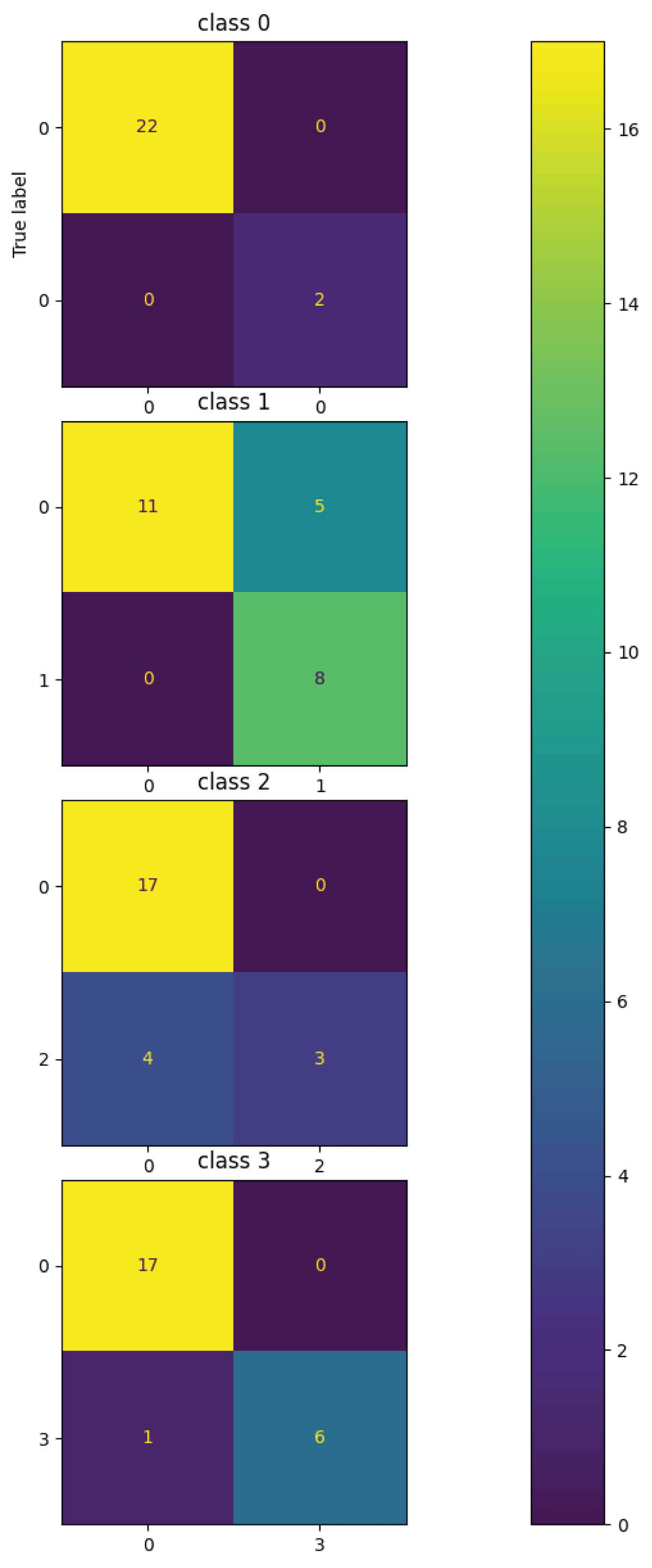
From Figure 4a, it can be said that the training loss is decreasing and the validation loss is fluctuating. After the completion of the training for fifty epochs, the training loss is 0.0015and the validation loss is 0.5771. So it can be said that the training loss is lower compared to the validation loss. Next from Figure 4b, it can be said that the training accuracy is increasing initially and then becomes constant. i.e. training accuracy increases initially till around ten epochs and then becomes constant around 1.00 after 10 epochs and remains at a value of 1.00 till 50 epochs. The validation accuracy increases in the beginning till around 10 epochs and then starts fluctuating around 0.80 after 10 epochs. So it can be observed that from Figure 4b, the training accuracy is greater than the validation accuracy i.e. the margin between the training accuracy and validation accuracy is more. So it can be said that the deep CNN model is Overfitting on the phase-only image dataset for the four-class classification task. The deep CNN model was tested using 24 phase-only images from the test set. Furthermore, the performance of the four-class classification task is illustrated by a multi-class confusion matrix. This matrix shows the number of images correctly and incorrectly classified for each class. Figure 5 presents the confusion matrix for the four classes, as obtained from the Deep CNN model on the phase-only image dataset. The multi-class classification task can be done for any number of classes. Here, four classes have been considered for the multi-class classification task. In general, n classes can be considered to perform multi-class classification tasks.

From Figure 5, it can be observed that the confusion matrix is represented for the four classes on the phase-only image dataset obtained from the deep CNN model. For Class-1, 22 images are predicted as FALSE and 2 as TRUE. For Class-2, 16 images are predicted as FALSE and 8 as TRUE. For Class-3, 17 images are predicted as FALSE and 7 as TRUE. Finally, for Class-4, 17 images are predicted as FALSE and 7 as TRUE. For Class 1, 22 images are recognized as true positive (TP), 2 images are recognized as true negative (TN), and finally 0 images are recognized as false positive (FP) and false negative (FN) respectively. For Class 2, 11 images are recognized as true negative (TN), 8 images as true positive (TP), 5 images as false positive (FP), and 0 images as false negative (FN) respectively. For Class 3, 17 images are recognized as true negative (TN), 3 images are recognized as true positive (TP), 4 images are recognized as false negative (FN), and 0 images as false positive (FP) respectively. For Class 4, 17 images are recognized as true negative (TN), 6 images are recognized as true positive (TP), 1 image as false negative (FN), and 0 images as false positive (FP) respectively. The performance metrics namely accuracy, positive predictive value (PPV), sensitivity, and F1-Score are calculated for all four classes namely Class 1, Class 2, Class 3, and Class 4 for both TRUE and FALSE classes. The metric accuracy is calculated by taking the ratio of the sum of true positives and true negatives to the sum of true positives, true negatives, false negatives, and false positives respectively. The metric positive predictive value is calculated by taking the ratio of true positives to the sum of true positives and false positives respectively. The metric sensitivity is calculated by taking the ratio of true positives to the sum of true positives and false negatives respectively. The metric F1-score is calculated by taking the ratio of the sum of twice of true positives to the sum of twice of true positives, false positives, and false negatives respectively. The metric mean squared error is calculated by taking the squared difference between ground truth and predicted values. The metric mean absolute error is calculated by taking the difference between the ground truth and the predicted values. The classification report from the deep CNN model for all four classes on the phase-only image dataset is shown in Table 1.

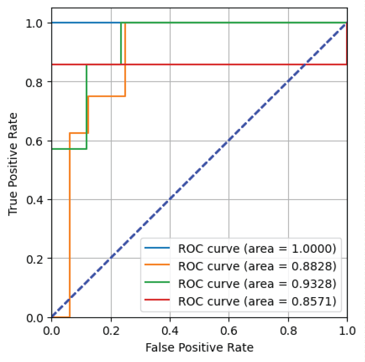
Table 1 highlights that the deep CNN model achieves higher accuracy for Class 1 compared to the other classes, with perfect (unity) values for Positive Predictive Value (PPV), sensitivity, and F1-score in both the FALSE and TRUE classes. The macro average is computed by averaging these metrics across TRUE and FALSE classes, while the weighted average combines macro and micro averages. For Class 1, the deep CNN model achieves unity values for both macro and weighted averages. In Class 2, the model demonstrates higher sensitivity but lower PPV for the TRUE class, and conversely, lower sensitivity and higher PPV for the FALSE class. The macro average results in the value of 0.81 for positive predictive value (PPV), 0.84 for sensitivity, and 0.79 for F1-score labels respectively. The weighted average results in the value of 0.87 for PPV, 0.79 for sensitivity, and 0.80 for F1-score labels respectively. The metrics mean squared error (MSE) and Mean Absolute Error (MAE) for the TRUE class are 0.12, and 0.12 for Classes 1 and 2 respectively. The deep CNN model has Classes 3 and 4 exhibits a pattern where PPV is higher but sensitivity is lower for the TRUE class compared to the FALSE class. In Class 3, the macro average results in the value of 0.90 for positive predictive value (PPV), 0.71 for sensitivity, and 0.75 for F1-score labels. The metric weighted average results in the value of 0.87 for PPV, 0.83 for sensitivity, and 0.81 for F1-score labels respectively. The mean square error (MSE) and Mean Absolute Error (MAE) values are 0.33, and 0.33 for Class 3 in the TRUE Class. In Class 4, the macro average results in the value of 0.97 for positive predictive value (PPV), 0.93 for sensitivity, and 0.95 for F1-score labels. The weighted average results in equal values for PPV, sensitivity, and F1-score labels respectively. i.e. 0.96 for PPV, sensitivity, and F1-score. The mean squared error and mean absolute error results in the values of 0.42, and 0.42 for Class 4 in the TRUE Class. Furthermore, the performance of the multi-class classification task is depicted using Receiver Operating Characteristic (ROC) curves and PPV-sensitivity characteristic curves in Figure 6. These curves illustrate how well the deep CNN model distinguishes between TRUE and FALSE classes, assessed by the area under the curve (AUC) metric.

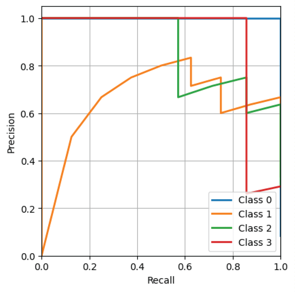
From Figure 6, it is evident that the deep CNN model has a higher AUC value for Class 1 compared to the other classes. Figure 7 displays the Positive Predictive Value (PPV) – sensitivity characteristic curve for all four classes obtained from the deep CNN model on the phase-only image dataset.

From Figure 7, it can be observed that the deep CNN model has higher sensitivity and lower positive predictive value for Class 4. Class 1 exhibits perfect positive predictive value and sensitivity on the phase-only image dataset from the deep CNN model. Classes 2 and 3 exhibit lower Positive Predictive Value (PPV) and higher sensitivity as depicted in Figure 7.

Conclusion

This paper presents a deep CNN-based approach for multi-class object classification, specifically focusing on a four-class classification task using phase-only digital holographic data obtained from phase-shifting digital holography (PSDH). The study involves four distinct 3-D objects: triangle-square, circle-square, square-triangle, and triangle-circle. Digital holograms of these objects are generated using a two-step PSDH technique and subsequently processed computationally to derive phase-reconstructed images. The dataset comprises 2880 phase-only images, which are utilized to train a deep CNN for classification purposes. The effectiveness of the proposed approach is demonstrated through various evaluation metrics. Loss and accuracy curves are presented to validate the efficacy of the model during training. Furthermore, results such as the confusion matrix, Receiver Operating Characteristic (ROC) curves, and Positive Predictive Value (PPV)-sensitivity curves are provided to substantiate the performance of the deep CNN in multi-class classification tasks using phase-shifting digital holographic data. This study underscores the application of deep learning as a modern and effective methodology for classifying 3-D objects based on phase-only holographic information. In the future, the deep CNN model can be used for live-cell images in the different forms of digital holographic information to perform binary classification and multi-class classification tasks.

References

1. Pitkäaho T, Manninen A, Naughton TJ. Focus prediction in digital holographic microscopy using deep convolutional neural networks. Appl Opt. 2019 Feb 10;58(5):A202-A208. doi: 10.1364/AO.58.00A202. PMID: 30873979.
2. Shimobaba T, Kakue T, Ito T. Convolutional neural network-based regression for depth prediction in digital holography. In: IEEE 27th International Symposium on Industrial Electronics (ISIE); 2018. p. 1323-1326. DOI: 10.1109/ISIE.2018.8433651.
3. Ronneberger O, Fischer P, Brox T. U-net: Convolutional networks for biomedical image segmentation. In: International Conference on Medical Image Computing and Computer-Assisted Intervention. Cham: Springer; 2015. p. 234-241. Available from: https://doi.org/10.1007/978-3-319-24574-4_28.
4. Wang K, Dou J, Kemao Q, Di J, Zhao J. Y-Net: a one-to-two deep learning framework for digital holographic reconstruction. Opt Lett. 2019 Oct 1;44(19):4765-4768. doi: 10.1364/OL.44.004765. PMID: 31568437.
5. Reddy BL, Mahesh RN, Nelleri A. Deep convolutional neural network for three-dimensional objects classification using off-axis digital Fresnel holography. J Mod Opt. 2022;69(13):705-717. Available from: https://doi.org/10.1080/09500340.2022.2081371.
6. Mahesh RNU, Nelleri A. Deep convolutional neural network for binary regression of three-dimensional objects using information retrieved from digital Fresnel holograms. Appl Phys B. 2022;128:157. Available from: https://doi.org/10.1007/s00340-022-07877-w.
7. Mahesh RNU, Nelleri A. Machine Learning-Based Binary Regression Task of 3D Objects in Digital Holography. In: Subhashini N, Ezra MAG, Liaw SK, editors. Futuristic Communication and Network Technologies. VICFCNT 2021. Lecture Notes in Electrical Engineering. Singapore: Springer; 2023. 995. Available from: https://doi.org/10.1007/978-981-19-9748-8_34.
8. Mahesh R N U, Nelleri A. Multi-Class Classification and Multi-Output Regression of Three-Dimensional Objects Using Artificial Intelligence Applied to Digital Holographic Information. Sensors (Basel). 2023 Jan 17;23(3):1095. doi: 10.3390/s23031095. PMID: 36772135; PMCID: PMC9920031.
9. Mahesh RN, Reddy BL, Nelleri A. Deep Learning-Based Multi-class 3D Objects Classification Using Digital Holographic Complex Images. In: Sivasubramanian A, Shastry PN, Hong PC, editors. Futuristic Communication and Network Technologies. VICFCNT 2020. Lecture Notes in Electrical Engineering, vol 792. Singapore: Springer; 2022. Available from: https://doi.org/10.1007/978-981-16-4625-6_43.
10. Mahesh RN, Nelleri A. Three-dimensional (3-D) objects classification and regression using deep learning and machine learning algorithms applied to complex object wave information retrieved from digital holograms. Asian J Phys. 2022;31(11-12):1085-1094.
11. Wang K, Li Y, Kemao Q, Di J, Zhao J. One-step robust deep learning phase unwrapping. Opt Express. 2019 May 13;27(10):15100-15115. doi: 10.1364/OE.27.015100. PMID: 31163947.
12. Li Z, Zhang L, Zhang Z, Xu R, Zhang D. Speckle classification of a multimode fiber based on Inception V3. Appl Opt. 2022 Oct 10;61(29):8850-8858. doi: 10.1364/AO.463764. PMID: 36256021.
13. Priscoli MD, Memmolo P, Ciaparrone G, Bianco V, Merola F, Miccio L, Bardozzo F, Pirone D, Mugnano M, Cimmino F, Capasso M. Raw holograms based machine learning for cancer cells classification in microfluidics. In: Digital Holography and Three-Dimensional Imaging. Optica Publishing Group; July 2021. p. DTh1D-3. Available from: https://doi.org/10.1364/DH.2021.DTh1D.3.
14. Lam HHS, Tsang PWM, Poon TC. Hologram classification of occluded and deformable objects with speckle noise contamination by deep learning. J Opt Soc Am A Opt Image Sci Vis. 2022 Mar 1;39(3):411-417. doi: 10.1364/JOSAA.444648. PMID: 35297424.
15. Cheng CJ, Chang Chien KC, Lin YC. Digital hologram for data augmentation in learning-based pattern classification. Opt Lett. 2018 Nov 1;43(21):5419-5422. doi: 10.1364/OL.43.005419. PMID: 30383022.
16. Zhang Y, Lu Y, Wang H, Chen P, Liang R. Automatic classification of marine plankton with digital holography using convolutional neural network. Opt Laser Technol. 2021;139:106979. Available from: https://doi.org/10.1016/j.optlastec.2021.106979.
17. Zhu Y, Yeung CH, Lam EY. Digital holography with deep learning and generative adversarial networks for automatic microplastics classification. In: Holography, Diffractive Optics, and Applications X. Vol 11551. SPIE; October 2020:22-27. Available from: https://doi.org/10.1117/12.2575115.

記事について